Basic Medical Data Exploration Visualization Heart Diseases
In this lecture we’re going to learn how to use matplotlib and seaborn by following along with the following example. As always, the source author’s link is listed for reference. This page will evolve over time.
Dataset
The dataset we’ll use here is the Heart Disease Data Set containing 302 patient data each with 75 attributes. However, this example only uses 14 of them which can be seen below.
The columns used include:
- age: age in years
- sex: sex
- 1 = male
- 0 = female
- cp: chest pain type
- Value 1: typical angina
- Value 2: atypical angina
- Value 3: non-anginal pain
- Value 4: asymptomatic
- trestbps: resting blood pressure (in mm Hg on admission to the hospital)
- chol: serum cholestoral in mg/dl
- fbs: fasting blood sugar > 120 mg/dl
- 1 = true
- 0 = false
- restecg: restecg: resting electrocardiographic results
- Value 0: normal
- Value 1: having ST-T wave abnormality (T wave inversions and/or ST elevation or depression of > 0.05 mV)
- Value 2: showing probable or definite left ventricular hypertrophy by Estes’ criteria
- thalach: maximum heart rate achieved
- exang: exercise induced angina
- 1 = yes
- 0 = no
- oldpeak: ST depression induced by exercise relative to rest
- slope: the slope of the peak exercise ST segment
- Value 1: upsloping
- Value 2: flat
- Value 3: downsloping
- ca: number of major vessels (0-3) colored by flourosopy
- thal:
- 3 = normal
- 6 = fixed defect
- 7 = reversable defect
- num: diagnosis of heart disease (angiographic disease status)
- Value 0: < 50% diameter narrowing
- Value 1: > 50% diameter narrowing
columns = ["age",
           "sex",
           "cp",
           "trestbps",
           "chol",
           "fbs",
           "restecg",
           "thalach",
           "exang",
           "oldpeak",
           "slope",
           "ca",
           "thal",
           "num"]
# disable warnings for lecture
import warnings
warnings.filterwarnings('ignore')
Overview of the Data Set , Cleaning, and Viewing
import pandas as pd

# import the data and see the basic description
df = pd.read_csv("https://archive.ics.uci.edu/ml/machine-learning-databases/heart-disease/processed.cleveland.data")
df.columns = columns
print("---- Describe ----")
print(df.describe())
---- Describe ----
              age         sex          cp    trestbps        chol         fbs  \
count  302.000000  302.000000  302.000000  302.000000  302.000000  302.000000
mean    54.410596    0.678808    3.165563  131.645695  246.738411    0.145695
std      9.040163    0.467709    0.953612   17.612202   51.856829    0.353386
min     29.000000    0.000000    1.000000   94.000000  126.000000    0.000000
25%     48.000000    0.000000    3.000000  120.000000  211.000000    0.000000
50%     55.500000    1.000000    3.000000  130.000000  241.500000    0.000000
75%     61.000000    1.000000    4.000000  140.000000  275.000000    0.000000
max     77.000000    1.000000    4.000000  200.000000  564.000000    1.000000

          restecg     thalach       exang     oldpeak       slope         num
count  302.000000  302.000000  302.000000  302.000000  302.000000  302.000000
mean     0.986755  149.605960    0.327815    1.035430    1.596026    0.940397
std      0.994916   22.912959    0.470196    1.160723    0.611939    1.229384
min      0.000000   71.000000    0.000000    0.000000    1.000000    0.000000
25%      0.000000  133.250000    0.000000    0.000000    1.000000    0.000000
50%      0.500000  153.000000    0.000000    0.800000    2.000000    0.000000
75%      2.000000  166.000000    1.000000    1.600000    2.000000    2.000000
max      2.000000  202.000000    1.000000    6.200000    3.000000    4.000000
print('---- Info -----')
print(df.info())
---- Info -----
<class 'pandas.core.frame.DataFrame'>
RangeIndex: 302 entries, 0 to 301
Data columns (total 14 columns):
 #   Column    Non-Null Count  Dtype
---  ------    --------------  -----
 0   age       302 non-null    float64
 1   sex       302 non-null    float64
 2   cp        302 non-null    float64
 3   trestbps  302 non-null    float64
 4   chol      302 non-null    float64
 5   fbs       302 non-null    float64
 6   restecg   302 non-null    float64
 7   thalach   302 non-null    float64
 8   exang     302 non-null    float64
 9   oldpeak   302 non-null    float64
 10  slope     302 non-null    float64
 11  ca        302 non-null    object
 12  thal      302 non-null    object
 13  num       302 non-null    int64
dtypes: float64(11), int64(1), object(2)
memory usage: 33.2+ KB
None
We notice above that the ca and thal data elements are objects which we’ll likely want to remap. Let’s take a look at the data.
df['thal'].unique()
array(['3.0', '7.0', '6.0', '?'], dtype=object)
df['ca'].unique()
array(['3.0', '2.0', '0.0', '1.0', '?'], dtype=object)
From the codebook above we see these are coded values that we can remap.
# Replace Every Number greater than 0 to 1 to mark heart disease
df.loc[df['num'] > 0 , 'num'] = 1
df.ca = pd.to_numeric(df.ca, errors='coerce').fillna(0)
df.thal = pd.to_numeric(df.thal, errors='coerce').fillna(0)
df['thal'].unique()
array([3., 7., 6., 0.])
df['ca'].unique()
array([3., 2., 0., 1.])
Now we can view the datatypes of the remapped data to float64 and int64.
print('---- Dtype ----')
print(df.dtypes)
---- Dtype ----
age         float64
sex         float64
cp          float64
trestbps    float64
chol        float64
fbs         float64
restecg     float64
thalach     float64
exang       float64
oldpeak     float64
slope       float64
ca          float64
thal        float64
num           int64
dtype: object
Next we’ll want to
print('---- Null Data ----')
# count how many null values exist
print(df.isnull().sum())
---- Null Data ----
age         0
sex         0
cp          0
trestbps    0
chol        0
fbs         0
restecg     0
thalach     0
exang       0
oldpeak     0
slope       0
ca          0
thal        0
num         0
dtype: int64
# quickly check to see if there are any null values
print(df.isnull().values.any())
False
After doing simple clean up, changing non-numerical value to NaN and replacing NaN with 0 we can safely say our data is somewhat clean.
First / Last 10 Rows
# print the first 10 and last 10
print('------ First 10 -------')
df.head(10)
------ First 10 -------
| age | sex | cp | trestbps | chol | fbs | restecg | thalach | exang | oldpeak | slope | ca | thal | num | |
|---|---|---|---|---|---|---|---|---|---|---|---|---|---|---|
| 0 | 67.0 | 1.0 | 4.0 | 160.0 | 286.0 | 0.0 | 2.0 | 108.0 | 1.0 | 1.5 | 2.0 | 3.0 | 3.0 | 1 |
| 1 | 67.0 | 1.0 | 4.0 | 120.0 | 229.0 | 0.0 | 2.0 | 129.0 | 1.0 | 2.6 | 2.0 | 2.0 | 7.0 | 1 |
| 2 | 37.0 | 1.0 | 3.0 | 130.0 | 250.0 | 0.0 | 0.0 | 187.0 | 0.0 | 3.5 | 3.0 | 0.0 | 3.0 | 0 |
| 3 | 41.0 | 0.0 | 2.0 | 130.0 | 204.0 | 0.0 | 2.0 | 172.0 | 0.0 | 1.4 | 1.0 | 0.0 | 3.0 | 0 |
| 4 | 56.0 | 1.0 | 2.0 | 120.0 | 236.0 | 0.0 | 0.0 | 178.0 | 0.0 | 0.8 | 1.0 | 0.0 | 3.0 | 0 |
| 5 | 62.0 | 0.0 | 4.0 | 140.0 | 268.0 | 0.0 | 2.0 | 160.0 | 0.0 | 3.6 | 3.0 | 2.0 | 3.0 | 1 |
| 6 | 57.0 | 0.0 | 4.0 | 120.0 | 354.0 | 0.0 | 0.0 | 163.0 | 1.0 | 0.6 | 1.0 | 0.0 | 3.0 | 0 |
| 7 | 63.0 | 1.0 | 4.0 | 130.0 | 254.0 | 0.0 | 2.0 | 147.0 | 0.0 | 1.4 | 2.0 | 1.0 | 7.0 | 1 |
| 8 | 53.0 | 1.0 | 4.0 | 140.0 | 203.0 | 1.0 | 2.0 | 155.0 | 1.0 | 3.1 | 3.0 | 0.0 | 7.0 | 1 |
| 9 | 57.0 | 1.0 | 4.0 | 140.0 | 192.0 | 0.0 | 0.0 | 148.0 | 0.0 | 0.4 | 2.0 | 0.0 | 6.0 | 0 |
#  Last 10
print('------ Last 10 -------')
df.tail(10)
------ Last 10 -------
| age | sex | cp | trestbps | chol | fbs | restecg | thalach | exang | oldpeak | slope | ca | thal | num | |
|---|---|---|---|---|---|---|---|---|---|---|---|---|---|---|
| 292 | 63.0 | 1.0 | 4.0 | 140.0 | 187.0 | 0.0 | 2.0 | 144.0 | 1.0 | 4.0 | 1.0 | 2.0 | 7.0 | 1 |
| 293 | 63.0 | 0.0 | 4.0 | 124.0 | 197.0 | 0.0 | 0.0 | 136.0 | 1.0 | 0.0 | 2.0 | 0.0 | 3.0 | 1 |
| 294 | 41.0 | 1.0 | 2.0 | 120.0 | 157.0 | 0.0 | 0.0 | 182.0 | 0.0 | 0.0 | 1.0 | 0.0 | 3.0 | 0 |
| 295 | 59.0 | 1.0 | 4.0 | 164.0 | 176.0 | 1.0 | 2.0 | 90.0 | 0.0 | 1.0 | 2.0 | 2.0 | 6.0 | 1 |
| 296 | 57.0 | 0.0 | 4.0 | 140.0 | 241.0 | 0.0 | 0.0 | 123.0 | 1.0 | 0.2 | 2.0 | 0.0 | 7.0 | 1 |
| 297 | 45.0 | 1.0 | 1.0 | 110.0 | 264.0 | 0.0 | 0.0 | 132.0 | 0.0 | 1.2 | 2.0 | 0.0 | 7.0 | 1 |
| 298 | 68.0 | 1.0 | 4.0 | 144.0 | 193.0 | 1.0 | 0.0 | 141.0 | 0.0 | 3.4 | 2.0 | 2.0 | 7.0 | 1 |
| 299 | 57.0 | 1.0 | 4.0 | 130.0 | 131.0 | 0.0 | 0.0 | 115.0 | 1.0 | 1.2 | 2.0 | 1.0 | 7.0 | 1 |
| 300 | 57.0 | 0.0 | 2.0 | 130.0 | 236.0 | 0.0 | 2.0 | 174.0 | 0.0 | 0.0 | 2.0 | 1.0 | 3.0 | 1 |
| 301 | 38.0 | 1.0 | 3.0 | 138.0 | 175.0 | 0.0 | 0.0 | 173.0 | 0.0 | 0.0 | 1.0 | 0.0 | 3.0 | 0 |
Plotting Histograms
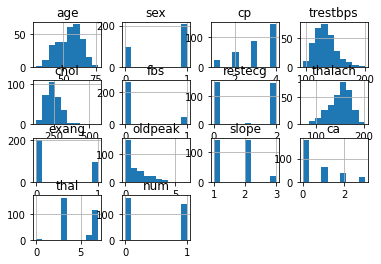
After reviewing the data in tabular form we want to visualize all of the data across the variables. We can do this easily with a histogram.
# import matplotlib
import matplotlib.pyplot as plt
%matplotlib inline
# using pandas to generate the plots
df.hist()

# using matplotlib to render (or show) the plot
plt.show()
# get the histogram of every data points
fig = plt.figure(figsize = (18, 18))
ax = fig.gca()

df.hist(ax=ax, bins=30)
plt.show()
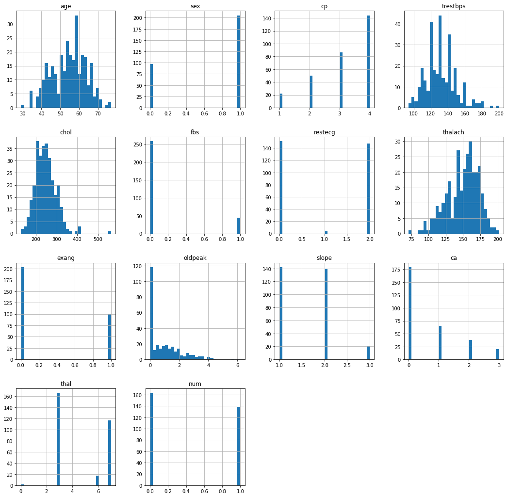
With simple histogram of our data, we can easily observe the distribution of different attributes. One thing to note here is the fact that it is extremely easy for us to see which attributes are categorical values and which are not.
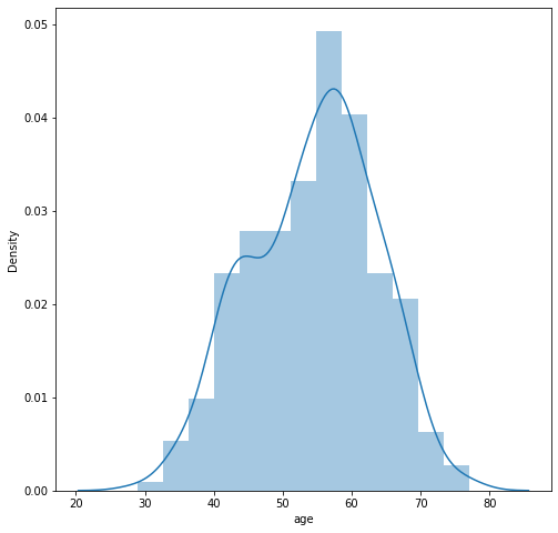
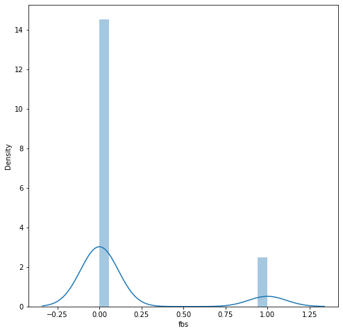
We can inspect a little bit more closely and take a look at the distribution of ages and fbs (fasting blood sugar). We can see that the age distribution is closely resembling of Gaussian distribution while fbs is a categorical value.
# import seaborn
import seaborn as sns

# a closer look at age
plt.figure(figsize=(8, 8))
sns.distplot(df.age)
plt.show()
plt.close('all')
# a closer look at fbs
plt.figure(figsize=(8, 8))
sns.distplot(df.fbs)
plt.show()
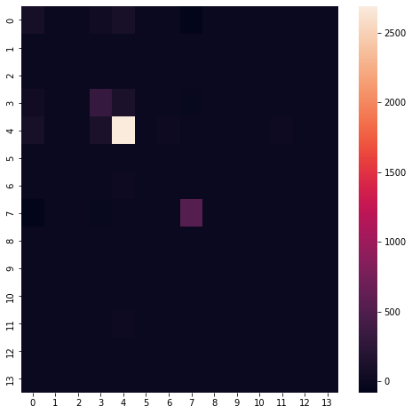
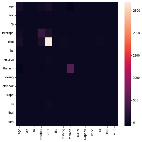
Variance-Covariance Matrix
We can calculate variance-covariance matrices in a number of ways. First we’ll use Numpy and then we’ll use the built-in Dataframe functrion. Once calculated, we can observe that most attributes do not have a strong covariance relationship.
import numpy as np
from numpy import dot

# calculate the Variance-Covariance Matrix
sample = df.values
sample = sample - dot(np.ones((sample.shape[0],sample.shape[0])),sample)/(len(sample)-1)
covv = dot(sample.T,sample)/(len(sample)-1)
plt.figure(figsize=(8,8))
sns.heatmap(covv)
plt.show()
# compare with built in
plt.figure(figsize=(8,8))
sns.heatmap(df.cov())
plt.show()
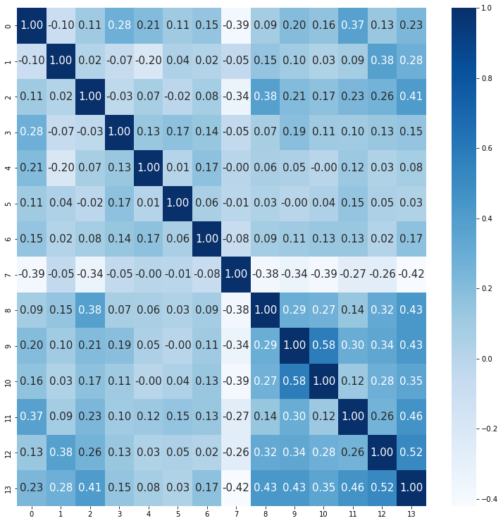
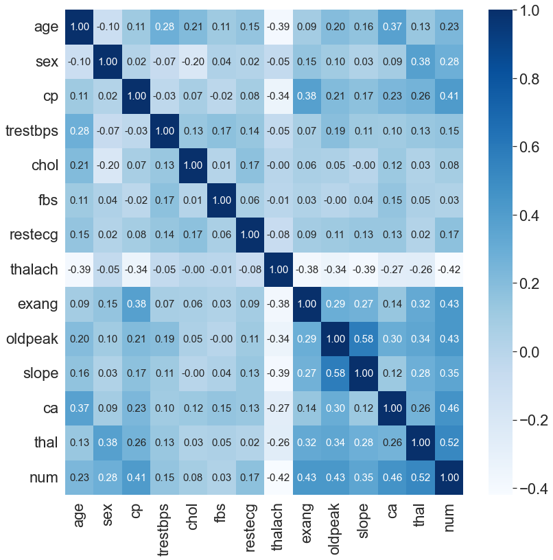
Correlation matrix
Similarly, the first image is created by manual numpy calculation and the second using the bulit-in method. Ee can observe that among the attributes there are actually strong correlation with one another. (especially heart disease and thal).
# calculate correaltion matrix
sample = df.values
certering_mat = np.diag(np.ones((302))) - np.ones((302,302))/302
std_matrix = np.diag(np.std(sample,0))
temp = dot(certering_mat,dot(sample, np.linalg.inv(std_matrix)  ))
temp = dot(temp.T,temp)/len(sample)

# plot
plt.figure(figsize=(13, 13))
sns.heatmap(np.around(temp,2),annot=True,fmt=".2f",cmap="Blues",annot_kws={"size": 15})
plt.show()
# correaltion matrix
sns.set(font_scale=2)
plt.figure(figsize=(13,13))

sns.heatmap(df.corr().round(2),annot=True,fmt=".2f",cmap="Blues",annot_kws={"size": 15})
plt.show()
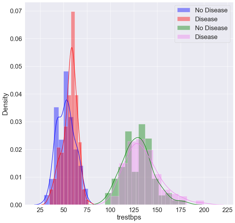
Interactive Histogram
# plot the people who have heart vs not
plt.figure(figsize=(13, 13))
sns.distplot(df.age[df.num==0], label='No Disease', color='blue')
sns.distplot(df.age[df.num==1], label='Disease', color='Red')
sns.distplot(df.trestbps[df.num==0],label= 'No Disease', color='Green')
sns.distplot(df.trestbps[df.num==1], label='Disease', color='violet')
plt.legend()
plt.show()
%matplotlib inline
import pygal
from IPython.display import SVG, HTML
html_pygal = """
<!DOCTYPE html>
<html>
  <head>
  <script type="text/javascript" src="http://kozea.github.com/pygal.js/javascripts/svg.jquery.js"></script>
  <script type="text/javascript" src="http://kozea.github.com/pygal.js/javascripts/pygal-tooltips.js"></script>
    <!-- ... -->
  </head>
  <body>
    <figure>
      {pygal_render}
    </figure>
  </body>
</html>
"""

hist = pygal.Histogram()

count, division = np.histogram(df.age[df.num==0].values,bins=100)
temp = []
for c,div in zip(count,division):
    temp.append((c,div,div+1))

count, division = np.histogram(df.age[df.num==1].values,bins=100)
temp1 = []
for c,div in zip(count,division):
    temp1.append((c,div,div+1))

count, division = np.histogram(df.trestbps[df.num==0].values,bins=100)
temp2 = []
for c,div in zip(count,division):
    temp2.append((c,div,div+1))

count, division = np.histogram(df.trestbps[df.num==1].values,bins=100)
temp3 = []
for c,div in zip(count,division):
    temp3.append((c,div,div+1))

hist.add('No Disease age', temp)
hist.add('Disease age', temp1)
hist.add('No Disease ', temp2)
hist.add('Disease', temp3)
hist.render()
HTML(html_pygal.format(pygal_render=hist.render()))
<!DOCTYPE html>