Python Numpy Array Tutorial

Source

A NumPy tutorial for beginners in which you’ll learn how to create a NumPy array, use broadcasting, access values, manipulate arrays, and much more.

NumPy is, just like SciPy, Scikit-Learn, Pandas, etc. one of the packages that you just can’t miss when you’re learning data science, mainly because this library provides you with an array data structure that holds some benefits over Python lists, such as: being more compact, faster access in reading and writing items, being more convenient and more efficient.

Today we’ll focus precisely on this. This NumPy tutorial will not only show you what NumPy arrays actually are and how you can install Python, but you’ll also learn how to make arrays (even when your data comes from files!), how broadcasting works, how you can ask for help, how to manipulate your arrays and how to visualize them.

Content

What Is A Python Numpy Array?
How To Make NumPy Arrays
How NumPy Broadcasting Works
How Do Array Mathematics Work?
How To Subset, Slice, And Index Arrays
How To Manipulate Arrays
How To Visualize NumPy Arrays
Beyond Data Analysis with NumPy

What Is A Python Numpy Array?

You already read in the introduction that NumPy arrays are a bit like Python lists, but still very much different at the same time. For those of you who are new to the topic, let’s clarify what it exactly is and what it’s good for.

As the name gives away, a NumPy array is a central data structure of the numpy library. The library’s name is short for “Numeric Python” or “Numerical Python”.

This already gives an idea of what you’re dealing with, right?

In other words, NumPy is a Python library that is the core library for scientific computing in Python. It contains a collection of tools and techniques that can be used to solve on a computer mathematical models of problems in Science and Engineering. One of these tools is a high-performance multidimensional array object that is a powerful data structure for efficient computation of arrays and matrices. To work with these arrays, there’s a vast amount of high-level mathematical functions operate on these matrices and arrays.

Then, what is an array?

When you look at the print of a couple of arrays, you could see it as a grid that contains values of the same type:

# import the library
import numpy as np

# create a 1-dimensional array
my_array = np.array([1, 2, 3, 4, 5, 6, 7, 8 ,9, 10, 11, 12])
print(type(my_array), my_array)

<class 'numpy.ndarray'> [ 1  2  3  4  5  6  7  8  9 10 11 12]

# create a 2-dimensional array
my_2d_array = np.array([[1, 2, 3, 4], [5, 6, 7, 8], [9, 10, 11, 12]])
print(my_2d_array)

[[ 1  2  3  4]
 [ 5  6  7  8]
 [ 9 10 11 12]]

# create a 3-dimensional array
my_3d_array = np.array([[[1, 2, 3, 4], [5, 6, 7, 8]], [[9, 10, 11, 12], [13, 14, 15, 16]]])
print(my_3d_array)

[[[ 1  2  3  4]
  [ 5  6  7  8]]

 [[ 9 10 11 12]
  [13 14 15 16]]]

You see that, in the example above, the data are integers. The array holds and represents any regular data in a structured way.

However, you should know that, on a structural level, an array is basically nothing but pointers. It’s a combination of a memory address, a data type, a shape, and strides:

The data pointer indicates the memory address of the first byte in the array,
The data type or dtype pointer describes the kind of elements that are contained within the array,
The shape indicates the shape of the array, and
The strides are the number of bytes that should be skipped in memory to go to the next element. If your strides are (10,1), you need to proceed one byte to get to the next column and 10 bytes to locate the next row.

Or, in other words, an array contains information about the raw data, how to locate an element and how to interpret an element.

You can easily test this by exploring the numpy array attributes:

# Print out memory address
print('Memory Address', my_2d_array.data)

# Print out the shape of `my_array`
print('Shape', my_2d_array.shape)

# Print out the data type of `my_array`
print('Data Type', my_2d_array.dtype)

# Print out the stride of `my_array`
print('Strides', my_2d_array.strides)

Memory Address <memory at 0x7faf50c48040>
Shape (3, 4)
Data Type int64
Strides (32, 8)

You see that now, you get a lot more information: for example, the data type that is printed out is ‘int64’ or signed 32-bit integer type; This is a lot more detailed! That also means that the array is stored in memory as 64 bytes (as each integer takes up 8 bytes and you have an array of 8 integers). The strides of the array tell us that you have to skip 8 bytes (one value) to move to the next column, but 32 bytes (4 values) to get to the same position in the next row. As such, the strides for the array will be (32,8).

Note that if you set the data type to int32, the strides tuple that you get back will be (16, 4), as you will still need to move one value to the next column and 4 values to get the same position. The only thing that will have changed is the fact that each integer will take up 4 bytes instead of 8.

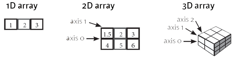
The array that you see above is, as its name already suggested, a 2-dimensional array: you have rows and columns. The rows are indicated as the “axis 0”, while the columns are the “axis 1”. The number of the axis goes up accordingly with the number of the dimensions: in 3-D arrays, of which you have also seen an example in the previous code chunk, you’ll have an additional “axis 2”. Note that these axes are only valid for arrays that have at least 2 dimensions, as there is no point in having this for 1-D arrays;

These axes will come in handy later when you’re manipulating the shape of your NumPy arrays.

How To Make NumPy Arrays

To make a numpy array, you can just use the np.array() function. All you need to do is pass a list to it, and optionally, you can also specify the data type of the data. If you want to know more about the possible data types that you can pick, go here or consider taking a brief look at DataCamp’s NumPy cheat sheet.

There’s no need to go and memorize these NumPy data types if you’re a new user; But you do have to know and care what data you’re dealing with. The data types are there when you need more control over how your data is stored in memory and on disk. Especially in cases where you’re working with extensive data, it’s good that you know to control the storage type.

Don’t forget that, in order to work with the np.array() function, you need to make sure that the numpy library is present in your environment. The NumPy library follows an import convention: when you import this library, you have to make sure that you import it as np. By doing this, you’ll make sure that other Pythonistas understand your code more easily.

In the following example you’ll create the my_array array that you have already played around with above:

# Import `numpy` as `np`
import numpy as np

# Make the array `my_array`
my_array = np.array([[1,2,3,4], [5,6,7,8]], dtype=np.int32)

# Print `my_array`
print(my_array, my_array.dtype)

[[1 2 3 4]
 [5 6 7 8]] int32

However, sometimes you don’t know what data you want to put in your array, or you want to import data into a numpy array from another source. In those cases, you’ll make use of initial placeholders or functions to load data from text into arrays, respectively.

The following sections will show you how to do this.

How To Make An “Empty” NumPy Array

What people often mean when they say that they are creating “empty” arrays is that they want to make use of initial placeholders, which you can fill up afterward. You can initialize arrays with ones or zeros, but you can also create arrays that get filled up with evenly spaced values, constant or random values.

However, you can still make a totally empty array, too.

Luckily for us, there are quite a lot of functions to make

Try it all out below!

# Create an array of ones
np.ones((3, 4))

array([[1., 1., 1., 1.],
       [1., 1., 1., 1.],
       [1., 1., 1., 1.]])

# Create an array of zeros
np.zeros((2, 3, 4), dtype=np.int16)

array([[[0, 0, 0, 0],
        [0, 0, 0, 0],
        [0, 0, 0, 0]],

       [[0, 0, 0, 0],
        [0, 0, 0, 0],
        [0, 0, 0, 0]]], dtype=int16)

# Create an array with random values
np.random.random((2, 2))

array([[0.30514961, 0.53408847],
       [0.5699706 , 0.14205311]])

# Create an empty array
np.empty((3, 2))

array([[1.72723371e-077, 1.72723371e-077],
       [1.38338381e-322, 0.00000000e+000],
       [0.00000000e+000, 0.00000000e+000]])

# Create a full array
np.full((2, 2), 6)

array([[6, 6],
       [6, 6]])

# Create an array of evenly-spaced values
print(np.arange(10, 31, 5))

[10 15 20 25 30]

# Create an array of evenly-spaced values
np.linspace(0, 2, 9)

array([0.  , 0.25, 0.5 , 0.75, 1.  , 1.25, 1.5 , 1.75, 2.  ])

For some, such as np.ones(), np.random.random(), np.empty(), np.full() or np.zeros() the only thing that you need to do in order to make arrays with ones or zeros is pass the shape of the array that you want to make. As an option to np.ones() and np.zeros(), you can also specify the data type. In the case of np.full(), you also have to specify the constant value that you want to insert into the array.
With np.linspace() and np.arange() you can make arrays of evenly spaced values. The difference between these two functions is that the last value of the three that are passed in the code chunk above designates either the step value for np.linspace() or a number of samples for np.arange(). What happens in the first is that you want, for example, an array of 9 values that lie between 0 and 2. For the latter, you specify that you want an array to start at 10 and per steps of 5, generate values for the array that you’re creating.
Remember that NumPy also allows you to create an identity array or matrix with np.eye() and np.identity(). An identity matrix is a square matrix of which all elements in the principal diagonal are ones, and all other elements are zeros. When you multiply a matrix with an identity matrix, the given matrix is left unchanged.

How To Load NumPy Arrays From Text

Creating arrays with the help of initial placeholders or with some example data is an excellent way of getting started with numpy. But when you want to get started with data analysis, you’ll need to load data from text files.

With that what you have seen up until now, you won’t really be able to do much. Make use of some specific functions to load data from your files, such as loadtxt() or genfromtxt().

Let’s say you have the following text files with data:

# Import your data
x, y, z = np.loadtxt('data.txt',
                    skiprows=1,
                    unpack=True)
print(x)
print(y)
print(z)

[0.2536 0.4839 0.1292 0.1781 0.6253 0.6253]
[0.1008 0.4536 0.6875 0.3049 0.3486 0.3486]
[0.3857 0.3561 0.5929 0.8928 0.8791 0.8791]

In the code above, you use loadtxt() to load the data in your environment. You see that the first argument that both functions take is the text file data.txt. Next, there are some specific arguments for each: in the first statement, you skip the first row, and you return the columns as separate arrays with unpack=True. This means that the values in column Value1 will be put in x, and so on.

Note that, in case you have comma-delimited data or if you want to specify the data type, there are also the arguments delimiter and dtype that you can add to the loadtxt() arguments.

my_array2 = np.genfromtxt('data2.txt',
                      skip_header=1,
                      filling_values=-999)
print(my_array2)

[[ 4.839e-01  4.536e-01  3.561e-01]
 [ 1.292e-01  6.875e-01 -9.990e+02]
 [ 1.781e-01  3.049e-01  8.928e-01]
 [-9.990e+02  5.801e-01  2.038e-01]
 [ 5.993e-01  4.357e-01  7.410e-01]]

You see that here, you resort to genfromtxt() to load the data. In this case, you have to handle some missing values that are indicated by the 'MISSING' strings. Since the genfromtxt() function converts character strings in numeric columns to nan, you can convert these values to other ones by specifying the filling_values argument. In this case, you choose to set the value of these missing values to -999.

If by any chance, you have values that don’t get converted to nan by genfromtxt(), there’s always the missing_values argument that allows you to specify what the missing values of your data exactly are.

But this is not all.

Tip: check out this page to see what other arguments you can add to import your data successfully.

You now might wonder what the difference between these two functions really is.

The examples indicated this maybe implicitly, but, in general, genfromtxt() gives you a little bit more flexibility; It’s more robust than loadtxt().

Let’s make this difference a little bit more practical: the latter, loadtxt(), only works when each row in the text file has the same number of values; So when you want to handle missing values easily, you’ll typically find it easier to use genfromtxt().

But this is definitely not the only reason.

A brief look on the number of arguments that genfromtxt() has to offer will teach you that there is really a lot more things that you can specify in your import, such as the maximum number of rows to read or the option to automatically strip white spaces from variables.

How To Save NumPy Arrays

Once you have done everything that you need to do with your arrays, you can also save them to a file. If you want to save the array to a text file, you can use the savetxt() function to do this:

x = np.arange(0.0, 5.0, 1.0)
print(x)
np.savetxt('test.out', x, delimiter=',')

[0. 1. 2. 3. 4.]

Remember that np.arange() creates a NumPy array of evenly-spaced values. The third value that you pass to this function is the step value.

There are, of course, other ways to save your NumPy arrays to text files. Check out the functions in the table below if you want to get your data to binary files or archives:

Method	Description
`save()`	Save an array to a binary file in NumPy .npy format
`savez()`	Save several arrays into an uncompressed .npz archive
`savez_compressed()`	Save several arrays into a compressed .npz archive

How To Inspect Your NumPy Arrays

Besides the array attributes that have been mentioned above, namely, data, shape, dtype and strides, there are some more that you can use to easily get to know more about your arrays. The ones that you might find interesting to use when you’re just starting out are the following:

# Print the number of `my_array`'s dimensions
print(my_array.ndim)

# Print the number of `my_array`'s elements
print(my_array.size)

# Print information about `my_array`'s memory layout
print(my_array.flags)

  C_CONTIGUOUS : True
  F_CONTIGUOUS : False
  OWNDATA : True
  WRITEABLE : True
  ALIGNED : True
  WRITEBACKIFCOPY : False
  UPDATEIFCOPY : False

# Print the length of one array element in bytes
print(my_array.itemsize)

# Print the total consumed bytes by `my_array`'s elements
print(my_array.nbytes)

Also note that, besides the attributes, you also have some other ways of gaining more information on and even tweaking your array slightly:

# Print the length of `my_array`
print(len(my_array))

# Change the data type of `my_array`
my_float_array = my_array.astype(float)
print(my_float_array)

[[1. 2. 3. 4.]
 [5. 6. 7. 8.]]

How NumPy Broadcasting Works

Before you go deeper into scientific computing, it might be a good idea to first go over what broadcasting exactly is: it’s a mechanism that allows NumPy to work with arrays of different shapes when you’re performing arithmetic operations.

To put it in a more practical context, you often have an array that’s somewhat larger and another one that’s slightly smaller. Ideally, you want to use the smaller array multiple times to perform an operation (such as a sum, multiplication, etc.) on the larger array.

To do this, you use the broadcasting mechanism.

However, there are some rules if you want to use it. And, before you already sigh, you’ll see that these “rules” are very simple and kind of straightforward!

First off, to make sure that the broadcasting is successful, the dimensions of your arrays need to be compatible. Two dimensions are compatible when they are equal. Consider the following example:

# Initialize `x`
x = np.ones((3, 4))

# Check shape of `x`
print(x.shape)
print(x)

# Initialize `y`
y = np.random.random((3, 4))

# Check shape of `y`
print(y.shape)
print(y)

# Add `x` and `y`
x + y

(3, 4)
[[1. 1. 1. 1.]
 [1. 1. 1. 1.]
 [1. 1. 1. 1.]]
(3, 4)
[[0.56519198 0.79797203 0.29302353 0.42378585]
 [0.20190445 0.37107571 0.50090031 0.36828103]
 [0.48683869 0.81527133 0.01208389 0.50830169]]





array([[1.56519198, 1.79797203, 1.29302353, 1.42378585],
       [1.20190445, 1.37107571, 1.50090031, 1.36828103],
       [1.48683869, 1.81527133, 1.01208389, 1.50830169]])

Two dimensions are also compatible when one of them is 1:

# Initialize `x`
x = np.ones((3, 4))

# Check shape of `x`
print(x.shape)
print(x)

# Initialize `y`
y = np.arange(4)

# Check shape of `y`
print(y.shape)
print(y)

# Subtract `x` and `y`
x - y 

(3, 4)
[[1. 1. 1. 1.]
 [1. 1. 1. 1.]
 [1. 1. 1. 1.]]
(4,)
[0 1 2 3]





array([[ 1.,  0., -1., -2.],
       [ 1.,  0., -1., -2.],
       [ 1.,  0., -1., -2.]])

Note that if the dimensions are not compatible, you will get a ValueError.

Tip: also test what the size of the resulting array is after you have done the computations! You’ll see that the size is actually the maximum size along each dimension of the input arrays.

In other words, you see that the result of x-y gives an array with shape (3,4): y had a shape of (4,) and x had a shape of (3,4). The maximum size along each dimension of x and y is taken to make up the shape of the new, resulting array.

Lastly, the arrays can only be broadcast together if they are compatible in all dimensions. Consider the following example:

# Initialize `x` and `y`
x = np.ones((3, 4))
y = np.random.random((5,1,4))

# Add `x` and `y`
x + y

array([[[1.83525793, 1.84535921, 1.23908934, 1.51636293],
        [1.83525793, 1.84535921, 1.23908934, 1.51636293],
        [1.83525793, 1.84535921, 1.23908934, 1.51636293]],

       [[1.96363415, 1.53040604, 1.28514896, 1.55804427],
        [1.96363415, 1.53040604, 1.28514896, 1.55804427],
        [1.96363415, 1.53040604, 1.28514896, 1.55804427]],

       [[1.40773584, 1.34067363, 1.26809999, 1.42783587],
        [1.40773584, 1.34067363, 1.26809999, 1.42783587],
        [1.40773584, 1.34067363, 1.26809999, 1.42783587]],

       [[1.24076123, 1.67608402, 1.70843067, 1.96111856],
        [1.24076123, 1.67608402, 1.70843067, 1.96111856],
        [1.24076123, 1.67608402, 1.70843067, 1.96111856]],

       [[1.46894321, 1.37966024, 1.56355702, 1.29747049],
        [1.46894321, 1.37966024, 1.56355702, 1.29747049],
        [1.46894321, 1.37966024, 1.56355702, 1.29747049]]])

You see that, even though x and y seem to have somewhat different dimensions, the two can be added together.

That is because they are compatible in all dimensions:

Array x has dimensions 3 X 4,
Array y has dimensions 5 X 1 X 4

Since you have seen above that dimensions are also compatible if one of them is equal to 1, you see that these two arrays are indeed a good candidate for broadcasting!

What you will notice is that in the dimension where y has size 1, and the other array has a size greater than 1 (that is, 3), the first array behaves as if it were copied along that dimension.

Note that the shape of the resulting array will again be the maximum size along each dimension of x and y: the dimension of the result will be (5,3,4)

In short, if you want to make use of broadcasting, you will rely a lot on the shape and dimensions of the arrays with which you’re working.

But what if the dimensions are not compatible?

What if they are not equal or if one of them is not equal to 1?

You’ll have to fix this by manipulating your array! You’ll see how to do this in one of the next sections.

How Do Array Mathematics Work?

You’ve seen that broadcasting is handy when you’re doing arithmetic operations. In this section, you’ll discover some of the functions that you can use to do mathematics with arrays.

As such, it probably won’t surprise you that you can just use +, -, *, / or % to add, subtract, multiply, divide or calculate the remainder of two (or more) arrays. However, a big part of why NumPy is so handy, is because it also has functions to do this. The equivalent functions of the operations that you have seen just now are, respectively, np.add(), np.subtract(), np.multiply(), np.divide() and np.remainder().

You can also easily do exponentiation and taking the square root of your arrays with np.exp() and np.sqrt(), or calculate the sines or cosines of your array with np.sin() and np.cos(). Lastly, its’ also useful to mention that there’s also a way for you to calculate the natural logarithm with np.log() or calculate the dot product by applying the dot() to your array.

# Add `x` and `y`
np.add(x, y)

array([[[1.83525793, 1.84535921, 1.23908934, 1.51636293],
        [1.83525793, 1.84535921, 1.23908934, 1.51636293],
        [1.83525793, 1.84535921, 1.23908934, 1.51636293]],

       [[1.96363415, 1.53040604, 1.28514896, 1.55804427],
        [1.96363415, 1.53040604, 1.28514896, 1.55804427],
        [1.96363415, 1.53040604, 1.28514896, 1.55804427]],

       [[1.40773584, 1.34067363, 1.26809999, 1.42783587],
        [1.40773584, 1.34067363, 1.26809999, 1.42783587],
        [1.40773584, 1.34067363, 1.26809999, 1.42783587]],

       [[1.24076123, 1.67608402, 1.70843067, 1.96111856],
        [1.24076123, 1.67608402, 1.70843067, 1.96111856],
        [1.24076123, 1.67608402, 1.70843067, 1.96111856]],

       [[1.46894321, 1.37966024, 1.56355702, 1.29747049],
        [1.46894321, 1.37966024, 1.56355702, 1.29747049],
        [1.46894321, 1.37966024, 1.56355702, 1.29747049]]])

# Subtract `x` and `y`
np.subtract(x, y)

array([[[0.16474207, 0.15464079, 0.76091066, 0.48363707],
        [0.16474207, 0.15464079, 0.76091066, 0.48363707],
        [0.16474207, 0.15464079, 0.76091066, 0.48363707]],

       [[0.03636585, 0.46959396, 0.71485104, 0.44195573],
        [0.03636585, 0.46959396, 0.71485104, 0.44195573],
        [0.03636585, 0.46959396, 0.71485104, 0.44195573]],

       [[0.59226416, 0.65932637, 0.73190001, 0.57216413],
        [0.59226416, 0.65932637, 0.73190001, 0.57216413],
        [0.59226416, 0.65932637, 0.73190001, 0.57216413]],

       [[0.75923877, 0.32391598, 0.29156933, 0.03888144],
        [0.75923877, 0.32391598, 0.29156933, 0.03888144],
        [0.75923877, 0.32391598, 0.29156933, 0.03888144]],

       [[0.53105679, 0.62033976, 0.43644298, 0.70252951],
        [0.53105679, 0.62033976, 0.43644298, 0.70252951],
        [0.53105679, 0.62033976, 0.43644298, 0.70252951]]])

# Multiply `x` and `y`
np.multiply(x, y)

array([[[0.83525793, 0.84535921, 0.23908934, 0.51636293],
        [0.83525793, 0.84535921, 0.23908934, 0.51636293],
        [0.83525793, 0.84535921, 0.23908934, 0.51636293]],

       [[0.96363415, 0.53040604, 0.28514896, 0.55804427],
        [0.96363415, 0.53040604, 0.28514896, 0.55804427],
        [0.96363415, 0.53040604, 0.28514896, 0.55804427]],

       [[0.40773584, 0.34067363, 0.26809999, 0.42783587],
        [0.40773584, 0.34067363, 0.26809999, 0.42783587],
        [0.40773584, 0.34067363, 0.26809999, 0.42783587]],

       [[0.24076123, 0.67608402, 0.70843067, 0.96111856],
        [0.24076123, 0.67608402, 0.70843067, 0.96111856],
        [0.24076123, 0.67608402, 0.70843067, 0.96111856]],

       [[0.46894321, 0.37966024, 0.56355702, 0.29747049],
        [0.46894321, 0.37966024, 0.56355702, 0.29747049],
        [0.46894321, 0.37966024, 0.56355702, 0.29747049]]])

# Divide `x` and `y`
np.divide(x, y)

array([[[1.19723497, 1.18292908, 4.18253694, 1.93662236],
        [1.19723497, 1.18292908, 4.18253694, 1.93662236],
        [1.19723497, 1.18292908, 4.18253694, 1.93662236]],

       [[1.03773824, 1.88534807, 3.50693892, 1.79197254],
        [1.03773824, 1.88534807, 3.50693892, 1.79197254],
        [1.03773824, 1.88534807, 3.50693892, 1.79197254]],

       [[2.45256831, 2.93536074, 3.72995169, 2.33734491],
        [2.45256831, 2.93536074, 3.72995169, 2.33734491],
        [2.45256831, 2.93536074, 3.72995169, 2.33734491]],

       [[4.15349266, 1.47910611, 1.41157073, 1.04045436],
        [4.15349266, 1.47910611, 1.41157073, 1.04045436],
        [4.15349266, 1.47910611, 1.41157073, 1.04045436]],

       [[2.13245436, 2.63393394, 1.77444335, 3.36167802],
        [2.13245436, 2.63393394, 1.77444335, 3.36167802],
        [2.13245436, 2.63393394, 1.77444335, 3.36167802]]])

# Calculate the remainder of `x` and `y`
np.remainder(x, y)

array([[[0.16474207, 0.15464079, 0.04364264, 0.48363707],
        [0.16474207, 0.15464079, 0.04364264, 0.48363707],
        [0.16474207, 0.15464079, 0.04364264, 0.48363707]],

       [[0.03636585, 0.46959396, 0.14455311, 0.44195573],
        [0.03636585, 0.46959396, 0.14455311, 0.44195573],
        [0.03636585, 0.46959396, 0.14455311, 0.44195573]],

       [[0.18452832, 0.31865274, 0.19570004, 0.14432825],
        [0.18452832, 0.31865274, 0.19570004, 0.14432825],
        [0.18452832, 0.31865274, 0.19570004, 0.14432825]],

       [[0.03695508, 0.32391598, 0.29156933, 0.03888144],
        [0.03695508, 0.32391598, 0.29156933, 0.03888144],
        [0.03695508, 0.32391598, 0.29156933, 0.03888144]],

       [[0.06211358, 0.24067951, 0.43644298, 0.10758854],
        [0.06211358, 0.24067951, 0.43644298, 0.10758854],
        [0.06211358, 0.24067951, 0.43644298, 0.10758854]]])

Remember how broadcasting works? Check out the dimensions and the shapes of both x and y in your IPython shell. Are the rules of broadcasting respected?

But there is more.

Check out this small list of aggregate functions:

Function	Description
`a.sum()`	Array-wise sum
`a.min()`	Array-wise minimum value
`b.max(axis=0)`	Maximum value of an array row
`b.cumsum(axis=1)`	Cumulative sum of the elements
`a.mean()`	Mean
`b.median()`	Median
`a.corrcoef()`	Correlation coefficient
`np.std(b)`	Standard deviation

Besides all of these functions, you might also find it useful to know that there are mechanisms that allow you to compare array elements. For example, if you want to check whether the elements of two arrays are the same, you might use the == operator. To check whether the array elements are smaller or bigger, you use the < or > operators.

This all seems quite straightforward, yes?

However, you can also compare entire arrays with each other! In this case, you use the np.array_equal() function. Just pass in the two arrays that you want to compare with each other, and you’re done.

Note that, besides comparing, you can also perform logical operations on your arrays. You can start with np.logical_or(), np.logical_not() and np.logical_and(). This basically works like your typical OR, NOT and AND logical operations;

In the simplest example, you use OR to see whether your elements are the same (for example, 1), or if one of the two array elements is 1. If both of them are 0, you’ll return FALSE. You would use AND to see whether your second element is also 1 and NOT to see if the second element differs from 1.

# `x` AND `y` 
np.logical_and(x, y)

array([[[ True,  True,  True,  True],
        [ True,  True,  True,  True],
        [ True,  True,  True,  True]],

       [[ True,  True,  True,  True],
        [ True,  True,  True,  True],
        [ True,  True,  True,  True]],

       [[ True,  True,  True,  True],
        [ True,  True,  True,  True],
        [ True,  True,  True,  True]],

       [[ True,  True,  True,  True],
        [ True,  True,  True,  True],
        [ True,  True,  True,  True]],

       [[ True,  True,  True,  True],
        [ True,  True,  True,  True],
        [ True,  True,  True,  True]]])

# `x` OR `y` 
np.logical_or(x, y)

array([[[ True,  True,  True,  True],
        [ True,  True,  True,  True],
        [ True,  True,  True,  True]],

       [[ True,  True,  True,  True],
        [ True,  True,  True,  True],
        [ True,  True,  True,  True]],

       [[ True,  True,  True,  True],
        [ True,  True,  True,  True],
        [ True,  True,  True,  True]],

       [[ True,  True,  True,  True],
        [ True,  True,  True,  True],
        [ True,  True,  True,  True]],

       [[ True,  True,  True,  True],
        [ True,  True,  True,  True],
        [ True,  True,  True,  True]]])

How To Subset, Slice, And Index Arrays

Besides mathematical operations, you might also consider taking just a part of the original array (or the resulting array) or just some array elements to use in further analysis or other operations. In such case, you will need to subset, slice and/or index your arrays.

These operations are very similar to when you perform them on Python lists. If you want to check out the similarities for yourself, or if you want a more elaborate explanation, you might consider checking out DataCamp’s Python list tutorial.

If you have no clue at all on how these operations work, it suffices for now to know these two basic things:

You use square brackets [] as the index operator, and
Generally, you pass integers to these square brackets, but you can also put a colon : or a combination of the colon with integers in it to designate the elements/rows/columns you want to select.

Besides from these two points, the easiest way to see how this all fits together is by looking at some examples of subsetting:

# Select the element at the 1st index
print(my_array[1])

[5 6 7 8]

# Select the element at row 1 column 2
print(my_2d_array[1][2])

# Select the element at row 1 column 2
print(my_2d_array[1,2])

# Select the element at row 1, column 2 and 
print(my_3d_array[1,1,2])

Something a little bit more advanced than subsetting, if you will, is slicing. Here, you consider not just particular values of your arrays, but you go to the level of rows and columns. You’re basically working with “regions” of data instead of pure “locations”.

# Select items at index 0 and 1
print(my_array[0:2])

[[1 2 3 4]
 [5 6 7 8]]

# Select items at row 0 and 1, column 1
print(my_2d_array[0:2,1])

[2 6]

# Select items at row 1
# This is the same as saying `my_3d_array[1,:,:]
print(my_3d_array[1,...])

[[ 9 10 11 12]
 [13 14 15 16]]

Lastly, there’s also indexing. When it comes to NumPy, there are boolean indexing and advanced or “fancy” indexing.

First up is boolean indexing. Here, instead of selecting elements, rows or columns based on index number, you select those values from your array that fulfill a certain condition.

# Try out a simple example
mask = my_array < 2
print(mask)
print()
print(my_array[mask])

[[ True False False False]
 [False False False False]]

[1]

print(my_array[my_array < 2])

[1]

# Try out a simple example
mask = my_array > 3
print(mask)
print(my_array[mask])

[[False False False  True]
 [ True  True  True  True]]
[4 5 6 7 8]

# Specify a condition
bigger_than_3 = (my_3d_array >= 3)

# Use the condition to index our 3d array
print(my_3d_array[bigger_than_3])

[ 3  4  5  6  7  8  9 10 11 12 13 14 15 16]

# Specify a condition
mask = (my_3d_array >= 3) & (my_3d_array < 10)

# Use the condition to index our 3d array
print(my_3d_array[mask])

[3 4 5 6 7 8 9]

Note that, to specify a condition, you can also make use of the logical operators | (OR) and & (AND). If you would want to rewrite the condition above in such a way (which would be inefficient, but I demonstrate it here for educational purposes :)), you would get bigger_than_3 = (my_3d_array > 3) | (my_3d_array == 3).

With the arrays that have been loaded in, there aren’t too many possibilities, but with arrays that contain for example, names or capitals, the possibilities could be endless!

When it comes to fancy indexing, that what you basically do with it is the following: you pass a list or an array of integers to specify the order of the subset of rows you want to select out of the original array.

# Select elements at (1,0), (0,1), (1,2) and (0,0)
print(my_2d_array[[1, 0, 1, 0],[0, 1, 2, 0]])

[5 2 7 1]

# Select a subset of the rows and columns
print(my_2d_array[[1, 0, 1, 0]][:,[0,1,2,0]])

[[5 6 7 5]
 [1 2 3 1]
 [5 6 7 5]
 [1 2 3 1]]

Now, the second statement might seem to make less sense to you at first sight. This is normal. It might make more sense if you break it down:

If you just execute my_2d_array[[1,0,1,0]], the result is the following:

my_2d_array[[1,0,1,0]]

array([[5, 6, 7, 8],
       [1, 2, 3, 4],
       [5, 6, 7, 8],
       [1, 2, 3, 4]])

What the second part, namely, [:,[0,1,2,0]], is tell you that you want to keep all the rows of this result, but that you want to change the order of the columns around a bit. You want to display the columns 0, 1, and 2 as they are right now, but you want to repeat column 0 as the last column instead of displaying column number 3. This will give you the following result:

my_2d_array[:,[0,1,2,0]]

array([[ 1,  2,  3,  1],
       [ 5,  6,  7,  5],
       [ 9, 10, 11,  9]])

How To Manipulate Arrays

Performing mathematical operations on your arrays is one of the things that you’ll be doing, but probably most importantly to make this and the broadcasting work is to know how to manipulate your arrays.

Below are some of the most common manipulations that you’ll be doing.

How To Transpose Your Arrays

What transposing your arrays actually does is permuting the dimensions of it. Or, in other words, you switch around the shape of the array. Let’s take a small example to show you the effect of transposition:

# Print `my_2d_array`
print(my_2d_array)

[[ 1  2  3  4]
 [ 5  6  7  8]
 [ 9 10 11 12]]

# Transpose `my_2d_array`
print(np.transpose(my_2d_array))

[[ 1  5  9]
 [ 2  6 10]
 [ 3  7 11]
 [ 4  8 12]]

# Or use `T` to transpose `my_2d_array`
print(my_2d_array.T)

[[ 1  5  9]
 [ 2  6 10]
 [ 3  7 11]
 [ 4  8 12]]

Reshaping Versus Resizing Your Arrays

You might have read in the broadcasting section that the dimensions of your arrays need to be compatible if you want them to be good candidates for arithmetic operations. But the question of what you should do when that is not the case, was not answered yet.

Well, this is where you get the answer!

What you can do if the arrays don’t have the same dimensions, is resize your array. You will then return a new array that has the shape that you passed to the np.resize() function. If you pass your original array together with the new dimensions, and if that new array is larger than the one that you originally had, the new array will be filled with copies of the original array that are repeated as many times as is needed.

However, if you just apply np.resize() to the array and you pass the new shape to it, the new array will be filled with zeros.

# Print the shape of `x`
print(x.shape)
print(x)

(3, 4)
[[1. 1. 1. 1.]
 [1. 1. 1. 1.]
 [1. 1. 1. 1.]]

# Resize `x` to ((6,4))
np.resize(x, (4, 3))

array([[1., 1., 1.],
       [1., 1., 1.],
       [1., 1., 1.],
       [1., 1., 1.]])

np.resize(x, (3, 4))

array([[1., 1., 1., 1.],
       [1., 1., 1., 1.],
       [1., 1., 1., 1.]])

Besides resizing, you can also reshape your array. This means that you give a new shape to an array without changing its data. The key to reshaping is to make sure that the total size of the new array is unchanged. If you take the example of array x that was used above, which has a size of 3 X 4 or 12, you have to make sure that the new array also has a size of 12.

If you want to calculate the size of an array with code, make sure to use the size attribute: x.size or x.reshape((2,6)).size:

# Print the size of `x` to see what's possible
print(x.size)

# Flatten `x`
z = x.ravel()

# Print `z`
print(z)

[1. 1. 1. 1. 1. 1. 1. 1. 1. 1. 1. 1.]

If all else fails, you can also append an array to your original one or insert or delete array elements to make sure that your dimensions fit with the other array that you want to use for your computations.

Another operation that you might keep handy when you’re changing the shape of arrays is ravel(). This function allows you to flatten your arrays. This means that if you ever have 2D, 3D or n-D arrays, you can just use this function to flatten it all out to a 1-D array.

How To Append Arrays

When you append arrays to your original array, they are “glued” to the end of that original array. If you want to make sure that what you append does not come at the end of the array, you might consider inserting it. Go to the next section if you want to know more.

Appending is a pretty easy thing to do thanks to the NumPy library; You can just make use of the np.append().

# Append a 1D array to your `my_array`
new_array = np.append(my_array, [7, 8, 9, 10, 11, 12])

# Print `new_array`
print(my_array)
print(new_array)

[[1 2 3 4]
 [5 6 7 8]]
[ 1  2  3  4  5  6  7  8  7  8  9 10 11 12]

# Append an extra column to your `my_2d_array`
new_2d_array = np.append(my_2d_array, [[7], [8], [9]], axis=1)

# Print `new_2d_array`
print(new_2d_array)

[[ 1  2  3  4  7]
 [ 5  6  7  8  8]
 [ 9 10 11 12  9]]

Note how, when you append an extra column to my_2d_array, the axis is specified. Remember that axis 1 indicates the columns, while axis 0 indicates the rows in 2-D arrays.

How To Insert And Delete Array Elements

Next to appending, you can also insert and delete array elements. As you might have guessed by now, the functions that will allow you to do these operations are np.insert() and np.delete():

# Insert `5` at index 1
np.insert(my_array, 1, 5)

array([1, 5, 2, 3, 4, 5, 6, 7, 8], dtype=int32)

# Delete the value at index 1
# np.delete(my_array,[1])

How To Join And Split Arrays

You can also ‘merge’ or join your arrays. There are a bunch of functions that you can use for that purpose and most of them are listed below.

Try them out, but also make sure to test out what the shape of the arrays is in the IPython shell. The arrays that have been loaded are x, my_array, my_resized_array and my_2d_array.

# Concatentate `my_array` and `x`
print(np.concatenate((my_array, x)))

[[1. 2. 3. 4.]
 [5. 6. 7. 8.]
 [1. 1. 1. 1.]
 [1. 1. 1. 1.]
 [1. 1. 1. 1.]]

# Stack arrays row-wise
print(np.vstack((my_array, my_2d_array)))

[[ 1  2  3  4]
 [ 5  6  7  8]
 [ 1  2  3  4]
 [ 5  6  7  8]
 [ 9 10 11 12]]

my_resized_array = np.array([[91, 92, 93, 94], 
                             [91, 92, 93, 94], 
                             [91, 92, 93, 94]])
print(my_resized_array)

[[91 92 93 94]
 [91 92 93 94]
 [91 92 93 94]]

# Stack arrays row-wise
print(np.r_[my_resized_array, my_2d_array])

[[91 92 93 94]
 [91 92 93 94]
 [91 92 93 94]
 [ 1  2  3  4]
 [ 5  6  7  8]
 [ 9 10 11 12]]

# Stack arrays horizontally
print(np.hstack((my_resized_array, my_2d_array)))

[[91 92 93 94  1  2  3  4]
 [91 92 93 94  5  6  7  8]
 [91 92 93 94  9 10 11 12]]

# Stack arrays column-wise
print(np.column_stack((my_resized_array, my_2d_array)))

[[91 92 93 94  1  2  3  4]
 [91 92 93 94  5  6  7  8]
 [91 92 93 94  9 10 11 12]]

# Stack arrays column-wise
print(np.c_[my_resized_array, my_2d_array])

[[91 92 93 94  1  2  3  4]
 [91 92 93 94  5  6  7  8]
 [91 92 93 94  9 10 11 12]]

You’ll note a few things as you go through the functions:

The number of dimensions needs to be the same if you want to concatenate two arrays with np.concatenate(). As such, if you want to concatenate an array with my_array, which is 1-D, you’ll need to make sure that the second array that you have, is also 1-D.
With np.vstack(), you effortlessly combine my_array with my_2d_array. You just have to make sure that, as you’re stacking the arrays row-wise, that the number of columns in both arrays is the same. As such, you could also add an array with shape (2,4) or (3,4) to my_2d_array, as long as the number of columns matches. Stated differently, the arrays must have the same shape along all but the first axis. The same holds also for when you want to use np.r[].
For np.hstack(), you have to make sure that the number of dimensions is the same and that the number of rows in both arrays is the same. That means that you could stack arrays such as (2,3) or (2,4) to my_2d_array, which itself as a shape of (2,4). Anything is possible as long as you make sure that the number of rows matches. This function is still supported by NumPy, but you should prefer np.concatenate() or np.stack().
With np.column_stack(), you have to make sure that the arrays that you input have the same first dimension. In this case, both shapes are the same, but if my_resized_array were to be (2,1) or (2,), the arrays still would have been stacked.
np.c_[] is another way to concatenate. Here also, the first dimension of both arrays needs to match.

When you have joined arrays, you might also want to split them at some point. Just like you can stack them horizontally, you can also do the same but then vertically. You use np.hsplit() and np.vsplit(), respectively:

my_stacked_array = np.r_[my_resized_array, my_2d_array]

# Split `my_stacked_array` horizontally at the 2nd index
print(np.hsplit(my_stacked_array, 2))

[array([[91, 92],
       [91, 92],
       [91, 92],
       [ 1,  2],
       [ 5,  6],
       [ 9, 10]]), array([[93, 94],
       [93, 94],
       [93, 94],
       [ 3,  4],
       [ 7,  8],
       [11, 12]])]

# Split `my_stacked_array` vertically at the 2nd index
print(np.vsplit(my_stacked_array, 2))

[array([[91, 92, 93, 94],
       [91, 92, 93, 94],
       [91, 92, 93, 94]]), array([[ 1,  2,  3,  4],
       [ 5,  6,  7,  8],
       [ 9, 10, 11, 12]])]

What you need to keep in mind when you’re using both of these split functions is probably the shape of your array. Let’s take the above case as an example: my_stacked_array has a shape of (2,8). If you want to select the index at which you want the split to occur, you have to keep the shape in mind.

How To Visualize NumPy Arrays

Lastly, something that will definitely come in handy is to know how you can plot your arrays. This can especially be handy in data exploration, but also in later stages of the data science workflow, when you want to visualize your arrays.

With np.histogram()

Contrary to what the function might suggest, the np.histogram() function doesn’t draw the histogram but it does compute the occurrences of the array that fall within each bin; This will determine the area that each bar of your histogram takes up.

What you pass to the np.histogram() function then is first the input data or the array that you’re working with. The array will be flattened when the histogram is computed.

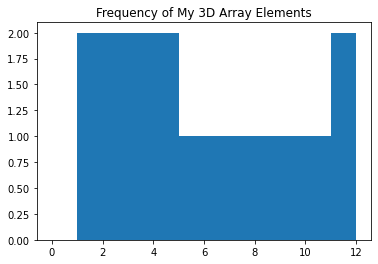
# Initialize your array
my_3d_array = np.array([[[1,2,3,4], [5,6,7,8]], [[1,2,3,4], [9,10,11,12]]], dtype=np.int64)

# Pass the array to `np.histogram()`
print(np.histogram(my_3d_array))

(array([4, 2, 2, 1, 1, 1, 1, 1, 1, 2]), array([ 1. ,  2.1,  3.2,  4.3,  5.4,  6.5,  7.6,  8.7,  9.8, 10.9, 12. ]))

# Specify the number of bins
print(np.histogram(my_3d_array, bins=range(0,13)))

(array([0, 2, 2, 2, 2, 1, 1, 1, 1, 1, 1, 2]), array([ 0,  1,  2,  3,  4,  5,  6,  7,  8,  9, 10, 11, 12]))

You’ll see that as a result, the histogram will be computed: the first array lists the frequencies for all the elements of your array, while the second array lists the bins that would be used if you don’t specify any bins.

If you do specify a number of bins, the result of the computation will be different: the floats will be gone and you’ll see all integers for the bins.

There are still some other arguments that you can specify that can influence the histogram that is computed. You can find all of them here.

But what is the point of computing such a histogram if you can’t visualize it?

Visualization is a piece of cake with the help of Matplotlib, but you don’t need np.histogram() to compute the histogram. plt.hist() does this for itself when you pass it the (flattened) data and the bins:

# Import numpy and matplotlib
import numpy as np
import matplotlib.pyplot as plt

# Construct the histogram with a flattened 3d array and a range of bins
plt.hist(my_3d_array.ravel(), bins=range(0,13))

# Add a title to the plot
plt.title('Frequency of My 3D Array Elements')

# Show the plot
plt.show()

png

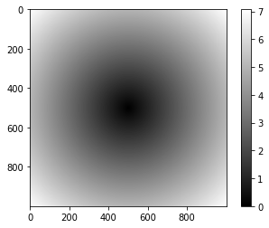
Using np.meshgrid()

Another way to (indirectly) visualize your array is by using np.meshgrid(). The problem that you face with arrays is that you need 2-D arrays of x and y coordinate values. With the above function, you can create a rectangular grid out of an array of x values and an array of y values: the np.meshgrid() function takes two 1D arrays and produces two 2D matrices corresponding to all pairs of (x, y) in the two arrays. Then, you can use these matrices to make all sorts of plots.

np.meshgrid() is particularly useful if you want to evaluate functions on a grid, as the code below demonstrates:

# Import NumPy and Matplotlib
import numpy as np
import matplotlib.pyplot as plt

# Create an array
points = np.arange(-5, 5, 0.01)

# Make a meshgrid
xs, ys = np.meshgrid(points, points)
z = np.sqrt(xs ** 2 + ys ** 2)

# Display the image on the axes
plt.imshow(z, cmap=plt.cm.gray)

# Draw a color bar
plt.colorbar()

# Show the plot
plt.show()

png