10 Minutes to pandas
This is a short introduction to pandas, geared mainly for new users. You can see more complex recipes in the Cookbook
Customarily, we import as follows:
import pandas as pd
import numpy as np
Object Creation
See the Data Structure Intro section
Creating a Series by passing a list of values, letting pandas create a default integer index:
s = pd.Series([1,3,5,np.nan,6,8])
s
0    1.0
1    3.0
2    5.0
3    NaN
4    6.0
5    8.0
dtype: float64
Creating a DataFrame by passing a numpy array, with a datetime index and labeled columns:
dates = pd.date_range('20130101', periods=6)
dates
DatetimeIndex(['2013-01-01', '2013-01-02', '2013-01-03', '2013-01-04',
               '2013-01-05', '2013-01-06'],
              dtype='datetime64[ns]', freq='D')
df = pd.DataFrame(np.random.randn(6,4), index=dates, columns=list('ABCD'))
df
| A | B | C | D | |
|---|---|---|---|---|
| 2013-01-01 | -0.534377 | -1.166835 | 0.552817 | 0.295235 |
| 2013-01-02 | -1.168310 | 0.852970 | -1.926660 | 0.271516 |
| 2013-01-03 | -0.494489 | -1.784271 | -0.122635 | -1.121595 |
| 2013-01-04 | -0.635309 | -0.263418 | 0.137195 | -0.353788 |
| 2013-01-05 | -0.771968 | -0.698785 | -1.119105 | 2.817852 |
| 2013-01-06 | 1.367584 | -1.239054 | -1.154439 | -0.714427 |
Creating a DataFrame by passing a dict of objects that can be converted to series-like.
df2 = pd.DataFrame({'A':1.,
                   'B':pd.Timestamp('20130102'),
                   'C':pd.Series(1,index=list(range(4)),dtype='float32'),
                   'D':np.array([3]*4,dtype='int32'),
                   'E':pd.Categorical(["test","train","test","train"]),
                   'F':'foo'})
df2
| A | B | C | D | E | F | |
|---|---|---|---|---|---|---|
| 0 | 1.0 | 2013-01-02 | 1.0 | 3 | test | foo |
| 1 | 1.0 | 2013-01-02 | 1.0 | 3 | train | foo |
| 2 | 1.0 | 2013-01-02 | 1.0 | 3 | test | foo |
| 3 | 1.0 | 2013-01-02 | 1.0 | 3 | train | foo |
The columns of the resulting DataFrame have different dtypes
df2.dtypes
A           float64
B    datetime64[ns]
C           float32
D             int32
E          category
F            object
dtype: object
If you’re using IPython, tab completion for column names (as well as public attributes) is automatically enabled. Here’s a subset of the attributes that will be completed:
# df2.<TAB>
As you can see, the columns A, B, C, and D are automatically tab completed. E is there as well; the rest of the attributes have been truncated for brevity.
Viewing Data
See the Basics section
Here is how to view the top and bottom rows of the frame:
df.head()
| A | B | C | D | |
|---|---|---|---|---|
| 2013-01-01 | -0.534377 | -1.166835 | 0.552817 | 0.295235 |
| 2013-01-02 | -1.168310 | 0.852970 | -1.926660 | 0.271516 |
| 2013-01-03 | -0.494489 | -1.784271 | -0.122635 | -1.121595 |
| 2013-01-04 | -0.635309 | -0.263418 | 0.137195 | -0.353788 |
| 2013-01-05 | -0.771968 | -0.698785 | -1.119105 | 2.817852 |
df.tail(3)
| A | B | C | D | |
|---|---|---|---|---|
| 2013-01-04 | -0.635309 | -0.263418 | 0.137195 | -0.353788 |
| 2013-01-05 | -0.771968 | -0.698785 | -1.119105 | 2.817852 |
| 2013-01-06 | 1.367584 | -1.239054 | -1.154439 | -0.714427 |
Display the index and columns
df.index
DatetimeIndex(['2013-01-01', '2013-01-02', '2013-01-03', '2013-01-04',
               '2013-01-05', '2013-01-06'],
              dtype='datetime64[ns]', freq='D')
df.columns
Index(['A', 'B', 'C', 'D'], dtype='object')
DataFrame.to_numpy() gives a NumPy representation of the underlying data. Note that this can be an expensive operation when your DataFrame has columns with different data types, which comes down to a fundamental difference between pandas and NumPy: NumPy arrays have one dtype for the entire array, while pandas DataFrames have one dtype per column. When you call DataFrame.to_numpy(), pandas will find the NumPy dtype that can hold all of the dtypes in the DataFrame. This may end up being object, which requires casting every value to a Python object.
For df, our DataFrame of all floating-point values, DataFrame.to_numpy() is fast and doesn’t require copying data.
df.to_numpy()
array([[-0.53437674, -1.16683512,  0.55281704,  0.29523502],
       [-1.1683095 ,  0.85296952, -1.92665959,  0.27151637],
       [-0.49448947, -1.7842706 , -0.12263523, -1.12159537],
       [-0.63530907, -0.26341834,  0.13719517, -0.35378752],
       [-0.77196761, -0.69878492, -1.11910468,  2.81785201],
       [ 1.36758353, -1.23905373, -1.15443949, -0.71442688]])
For df2, the DataFrame with multiple dtypes, DataFrame.to_numpy() is relatively expensive.
df2.to_numpy()
array([[1.0, Timestamp('2013-01-02 00:00:00'), 1.0, 3, 'test', 'foo'],
       [1.0, Timestamp('2013-01-02 00:00:00'), 1.0, 3, 'train', 'foo'],
       [1.0, Timestamp('2013-01-02 00:00:00'), 1.0, 3, 'test', 'foo'],
       [1.0, Timestamp('2013-01-02 00:00:00'), 1.0, 3, 'train', 'foo']],
      dtype=object)
describe shows a quick statistic summary of your data
df.describe()
| A | B | C | D | |
|---|---|---|---|---|
| count | 6.000000 | 6.000000 | 6.000000 | 6.000000 |
| mean | -0.372811 | -0.716566 | -0.605471 | 0.199132 |
| std | 0.886671 | 0.925725 | 0.942023 | 1.396911 |
| min | -1.168310 | -1.784271 | -1.926660 | -1.121595 |
| 25% | -0.737803 | -1.220999 | -1.145606 | -0.624267 |
| 50% | -0.584843 | -0.932810 | -0.620870 | -0.041136 |
| 75% | -0.504461 | -0.372260 | 0.072238 | 0.289305 |
| max | 1.367584 | 0.852970 | 0.552817 | 2.817852 |
Transposing your data
df.T
| 2013-01-01 | 2013-01-02 | 2013-01-03 | 2013-01-04 | 2013-01-05 | 2013-01-06 | |
|---|---|---|---|---|---|---|
| A | -0.534377 | -1.168310 | -0.494489 | -0.635309 | -0.771968 | 1.367584 |
| B | -1.166835 | 0.852970 | -1.784271 | -0.263418 | -0.698785 | -1.239054 |
| C | 0.552817 | -1.926660 | -0.122635 | 0.137195 | -1.119105 | -1.154439 |
| D | 0.295235 | 0.271516 | -1.121595 | -0.353788 | 2.817852 | -0.714427 |
Sorting by an axis
df.sort_index(axis=1, ascending=False)
| D | C | B | A | |
|---|---|---|---|---|
| 2013-01-01 | 0.295235 | 0.552817 | -1.166835 | -0.534377 |
| 2013-01-02 | 0.271516 | -1.926660 | 0.852970 | -1.168310 |
| 2013-01-03 | -1.121595 | -0.122635 | -1.784271 | -0.494489 |
| 2013-01-04 | -0.353788 | 0.137195 | -0.263418 | -0.635309 |
| 2013-01-05 | 2.817852 | -1.119105 | -0.698785 | -0.771968 |
| 2013-01-06 | -0.714427 | -1.154439 | -1.239054 | 1.367584 |
Sorting by value
df.sort_values(by='B')
| A | B | C | D | |
|---|---|---|---|---|
| 2013-01-03 | -0.494489 | -1.784271 | -0.122635 | -1.121595 |
| 2013-01-06 | 1.367584 | -1.239054 | -1.154439 | -0.714427 |
| 2013-01-01 | -0.534377 | -1.166835 | 0.552817 | 0.295235 |
| 2013-01-05 | -0.771968 | -0.698785 | -1.119105 | 2.817852 |
| 2013-01-04 | -0.635309 | -0.263418 | 0.137195 | -0.353788 |
| 2013-01-02 | -1.168310 | 0.852970 | -1.926660 | 0.271516 |
Selection
Note: While standard Python / Numpy expressions for selecting and setting are intuitive and come in handy for interactive work, for production code, we recommend the optimized pandas data access methods, .at, .iat, .loc, .iloc.
See the indexing documentation Indexing and Selecting Data and MultiIndex / Advanced Indexing
Getting
Selecting a single column, which yields a Series, equivalent to df.A
df['A']
2013-01-01   -0.534377
2013-01-02   -1.168310
2013-01-03   -0.494489
2013-01-04   -0.635309
2013-01-05   -0.771968
2013-01-06    1.367584
Freq: D, Name: A, dtype: float64
Selecting via [], which slices the rows.
df[0:3]
| A | B | C | D | |
|---|---|---|---|---|
| 2013-01-01 | -0.534377 | -1.166835 | 0.552817 | 0.295235 |
| 2013-01-02 | -1.168310 | 0.852970 | -1.926660 | 0.271516 |
| 2013-01-03 | -0.494489 | -1.784271 | -0.122635 | -1.121595 |
df['20130102':'20130104']
| A | B | C | D | |
|---|---|---|---|---|
| 2013-01-02 | -1.168310 | 0.852970 | -1.926660 | 0.271516 |
| 2013-01-03 | -0.494489 | -1.784271 | -0.122635 | -1.121595 |
| 2013-01-04 | -0.635309 | -0.263418 | 0.137195 | -0.353788 |
Selection by Label
See more in Selection by Label
For getting a cross section using a label:
df.loc[dates[0]]
A   -0.534377
B   -1.166835
C    0.552817
D    0.295235
Name: 2013-01-01 00:00:00, dtype: float64
Selecting on a multi-axis by label:
df.loc[:,['A','B']]
| A | B | |
|---|---|---|
| 2013-01-01 | -0.534377 | -1.166835 |
| 2013-01-02 | -1.168310 | 0.852970 |
| 2013-01-03 | -0.494489 | -1.784271 |
| 2013-01-04 | -0.635309 | -0.263418 |
| 2013-01-05 | -0.771968 | -0.698785 |
| 2013-01-06 | 1.367584 | -1.239054 |
Showing label slicing, both endpoints are included
df.loc['20130102':'20130104',['A','B']]
| A | B | |
|---|---|---|
| 2013-01-02 | -1.168310 | 0.852970 |
| 2013-01-03 | -0.494489 | -1.784271 |
| 2013-01-04 | -0.635309 | -0.263418 |
Reduction in the dimensions of the returned object
df.loc['20130102',['A','B']]
A   -1.16831
B    0.85297
Name: 2013-01-02 00:00:00, dtype: float64
For getting fast access to a scalar (equivalent to the prior method):
df.loc[dates[0],'A']
-0.5343767371269155
Selection by Position
See more in Selection by Position
Select via the position of the passed integers
df.iloc[3]
A   -0.635309
B   -0.263418
C    0.137195
D   -0.353788
Name: 2013-01-04 00:00:00, dtype: float64
By integer slices, acting similar to numpy/python
df.iloc[3:5,0:2]
| A | B | |
|---|---|---|
| 2013-01-04 | -0.635309 | -0.263418 |
| 2013-01-05 | -0.771968 | -0.698785 |
By lists of integer position locations, similar to the numpy/python style
df.iloc[[1,2,4],[0,2]]
| A | C | |
|---|---|---|
| 2013-01-02 | -1.168310 | -1.926660 |
| 2013-01-03 | -0.494489 | -0.122635 |
| 2013-01-05 | -0.771968 | -1.119105 |
For slicing rows explicitly
df.iloc[1:3,:]
| A | B | C | D | |
|---|---|---|---|---|
| 2013-01-02 | -1.168310 | 0.852970 | -1.926660 | 0.271516 |
| 2013-01-03 | -0.494489 | -1.784271 | -0.122635 | -1.121595 |
For slicing columns explicitly
df.iloc[:,1:3]
| B | C | |
|---|---|---|
| 2013-01-01 | -1.166835 | 0.552817 |
| 2013-01-02 | 0.852970 | -1.926660 |
| 2013-01-03 | -1.784271 | -0.122635 |
| 2013-01-04 | -0.263418 | 0.137195 |
| 2013-01-05 | -0.698785 | -1.119105 |
| 2013-01-06 | -1.239054 | -1.154439 |
For getting a value explicitly
df.iloc[1,1]
0.8529695184142756
For getting fast access to a scalar (equiv to the prior method)
df.iat[1,1]
0.8529695184142756
Boolean Indexing
Using a single column’s values to select data.
df[df["A"] > 0]
| A | B | C | D | |
|---|---|---|---|---|
| 2013-01-06 | 1.367584 | -1.239054 | -1.154439 | -0.714427 |
Selecting values from a DataFrame where a boolean condition is met.
df[df > 0]
| A | B | C | D | |
|---|---|---|---|---|
| 2013-01-01 | NaN | NaN | 0.552817 | 0.295235 |
| 2013-01-02 | NaN | 0.85297 | NaN | 0.271516 |
| 2013-01-03 | NaN | NaN | NaN | NaN |
| 2013-01-04 | NaN | NaN | 0.137195 | NaN |
| 2013-01-05 | NaN | NaN | NaN | 2.817852 |
| 2013-01-06 | 1.367584 | NaN | NaN | NaN |
Using the isin() method for filtering:
df2 = df.copy()
df2['E'] = ['one','one', 'two','three','four','three']
df2
| A | B | C | D | E | |
|---|---|---|---|---|---|
| 2013-01-01 | -0.534377 | -1.166835 | 0.552817 | 0.295235 | one |
| 2013-01-02 | -1.168310 | 0.852970 | -1.926660 | 0.271516 | one |
| 2013-01-03 | -0.494489 | -1.784271 | -0.122635 | -1.121595 | two |
| 2013-01-04 | -0.635309 | -0.263418 | 0.137195 | -0.353788 | three |
| 2013-01-05 | -0.771968 | -0.698785 | -1.119105 | 2.817852 | four |
| 2013-01-06 | 1.367584 | -1.239054 | -1.154439 | -0.714427 | three |
df2[df2['E'].isin(['two','four'])]
| A | B | C | D | E | |
|---|---|---|---|---|---|
| 2013-01-03 | -0.494489 | -1.784271 | -0.122635 | -1.121595 | two |
| 2013-01-05 | -0.771968 | -0.698785 | -1.119105 | 2.817852 | four |
Setting
Setting a new column automatically aligns the data by the indexes
s1 = pd.Series([1,2,3,4,5,6], index=pd.date_range('20130102',periods=6))
s1
2013-01-02    1
2013-01-03    2
2013-01-04    3
2013-01-05    4
2013-01-06    5
2013-01-07    6
Freq: D, dtype: int64
df['F'] = s1
Setting values by label
df.at[dates[0],'A'] = 0
Settomg values by position
df.iat[0,1] = 0
Setting by assigning with a numpy array
df.loc[:,'D'] = np.array([5] * len(df))
The result of the prior setting operations
df
| A | B | C | D | F | |
|---|---|---|---|---|---|
| 2013-01-01 | 0.000000 | 0.000000 | 0.552817 | 5 | NaN |
| 2013-01-02 | -1.168310 | 0.852970 | -1.926660 | 5 | 1.0 |
| 2013-01-03 | -0.494489 | -1.784271 | -0.122635 | 5 | 2.0 |
| 2013-01-04 | -0.635309 | -0.263418 | 0.137195 | 5 | 3.0 |
| 2013-01-05 | -0.771968 | -0.698785 | -1.119105 | 5 | 4.0 |
| 2013-01-06 | 1.367584 | -1.239054 | -1.154439 | 5 | 5.0 |
A where operation with setting.
df2 = df.copy()
df2[df2 > 0] = -df2
df2
| A | B | C | D | F | |
|---|---|---|---|---|---|
| 2013-01-01 | 0.000000 | 0.000000 | -0.552817 | -5 | NaN |
| 2013-01-02 | -1.168310 | -0.852970 | -1.926660 | -5 | -1.0 |
| 2013-01-03 | -0.494489 | -1.784271 | -0.122635 | -5 | -2.0 |
| 2013-01-04 | -0.635309 | -0.263418 | -0.137195 | -5 | -3.0 |
| 2013-01-05 | -0.771968 | -0.698785 | -1.119105 | -5 | -4.0 |
| 2013-01-06 | -1.367584 | -1.239054 | -1.154439 | -5 | -5.0 |
Missing Data
pandas primarily uses the value np.nan to represent missing data. It is by default not included in computations. See the Missing Data section
Reindexing allows you to change/add/delete the index on a specified axis. This returns a copy of the data.
df1 = df.reindex(index=dates[0:4], columns=list(df.columns) + ['E'])
df1.loc[dates[0]:dates[1],'E'] = 1
df1
| A | B | C | D | F | E | |
|---|---|---|---|---|---|---|
| 2013-01-01 | 0.000000 | 0.000000 | 0.552817 | 5 | NaN | 1.0 |
| 2013-01-02 | -1.168310 | 0.852970 | -1.926660 | 5 | 1.0 | 1.0 |
| 2013-01-03 | -0.494489 | -1.784271 | -0.122635 | 5 | 2.0 | NaN |
| 2013-01-04 | -0.635309 | -0.263418 | 0.137195 | 5 | 3.0 | NaN |
To drop any rows that have missing data.
df1.dropna(how='any')
| A | B | C | D | F | E | |
|---|---|---|---|---|---|---|
| 2013-01-02 | -1.16831 | 0.85297 | -1.92666 | 5 | 1.0 | 1.0 |
Filling missing data
df1.fillna(value=5)
| A | B | C | D | F | E | |
|---|---|---|---|---|---|---|
| 2013-01-01 | 0.000000 | 0.000000 | 0.552817 | 5 | 5.0 | 1.0 |
| 2013-01-02 | -1.168310 | 0.852970 | -1.926660 | 5 | 1.0 | 1.0 |
| 2013-01-03 | -0.494489 | -1.784271 | -0.122635 | 5 | 2.0 | 5.0 |
| 2013-01-04 | -0.635309 | -0.263418 | 0.137195 | 5 | 3.0 | 5.0 |
To get the boolean mask where values are nan
pd.isnull(df1)
| A | B | C | D | F | E | |
|---|---|---|---|---|---|---|
| 2013-01-01 | False | False | False | False | True | False |
| 2013-01-02 | False | False | False | False | False | False |
| 2013-01-03 | False | False | False | False | False | True |
| 2013-01-04 | False | False | False | False | False | True |
Operations
See the Basic section on Binary Ops
Stats
Operations in general exclude missing data.
Performing a descriptive statistic
df.mean()
A   -0.283749
B   -0.522093
C   -0.605471
D    5.000000
F    3.000000
dtype: float64
Same operation on the other axis
df.mean(1)
2013-01-01    1.388204
2013-01-02    0.751600
2013-01-03    0.919721
2013-01-04    1.447694
2013-01-05    1.282029
2013-01-06    1.794818
Freq: D, dtype: float64
Operating with objects that have different dimensionality and need alignment. In addition, pandas automatically broadcasts along the specified dimension.
s = pd.Series([1,3,5,np.nan,6,8], index=dates).shift(2)
s
2013-01-01    NaN
2013-01-02    NaN
2013-01-03    1.0
2013-01-04    3.0
2013-01-05    5.0
2013-01-06    NaN
Freq: D, dtype: float64
df.sub(s, axis='index')
| A | B | C | D | F | |
|---|---|---|---|---|---|
| 2013-01-01 | NaN | NaN | NaN | NaN | NaN |
| 2013-01-02 | NaN | NaN | NaN | NaN | NaN |
| 2013-01-03 | -1.494489 | -2.784271 | -1.122635 | 4.0 | 1.0 |
| 2013-01-04 | -3.635309 | -3.263418 | -2.862805 | 2.0 | 0.0 |
| 2013-01-05 | -5.771968 | -5.698785 | -6.119105 | 0.0 | -1.0 |
| 2013-01-06 | NaN | NaN | NaN | NaN | NaN |
Apply
Applying functions to the data
df.apply(np.cumsum)
| A | B | C | D | F | |
|---|---|---|---|---|---|
| 2013-01-01 | 0.000000 | 0.000000 | 0.552817 | 5 | NaN |
| 2013-01-02 | -1.168310 | 0.852970 | -1.373843 | 10 | 1.0 |
| 2013-01-03 | -1.662799 | -0.931301 | -1.496478 | 15 | 3.0 |
| 2013-01-04 | -2.298108 | -1.194719 | -1.359283 | 20 | 6.0 |
| 2013-01-05 | -3.070076 | -1.893504 | -2.478387 | 25 | 10.0 |
| 2013-01-06 | -1.702492 | -3.132558 | -3.632827 | 30 | 15.0 |
df.apply(lambda x: x.max() - x.min())
A    2.535893
B    2.637240
C    2.479477
D    0.000000
F    4.000000
dtype: float64
Histogramming
See more at Histogramming and Discretization
s = pd.Series(np.random.randint(0, 7, size=10))
s
0    2
1    6
2    6
3    0
4    1
5    6
6    3
7    0
8    4
9    3
dtype: int64
s.value_counts()
6    3
0    2
3    2
2    1
1    1
4    1
dtype: int64
String Methods
Series is equipped with a set of string processing methods in the str attribute that make it easy to operate on each element of the array, as in the code snippet below. Note that pattern-matching in str generally uses regular expressions by default (and in some cases always uses them). See more at Vectorized String Methods.
s = pd.Series(['A', 'B', 'C', 'Aaba', 'Baca', np.nan, 'CABA', 'dog', 'cat'])
s.str.lower()
0       a
1       b
2       c
3    aaba
4    baca
5     NaN
6    caba
7     dog
8     cat
dtype: object
Merge
Concat
pandas provides various facilities for easily combining together Series, DataFrame, and Panel objects with various kinds of set logic for the indexes and relational algebra functionality in the case of join / merge-type operations.
See the Merging section
Concatenating pandas objects together with concat():
df = pd.DataFrame(np.random.randn(10, 4))
df
| 0 | 1 | 2 | 3 | |
|---|---|---|---|---|
| 0 | -0.162034 | 0.087086 | -0.142747 | 0.558215 |
| 1 | -0.548816 | -0.803596 | 1.334449 | 0.847867 |
| 2 | -0.001181 | 1.259244 | -0.325483 | 0.138625 |
| 3 | 0.880145 | 1.878703 | 0.217188 | -0.343998 |
| 4 | 1.372847 | -0.923290 | -0.284173 | -0.869420 |
| 5 | 0.399153 | -1.378420 | 1.009660 | 1.317131 |
| 6 | -0.657825 | -1.498784 | 1.135572 | 0.450978 |
| 7 | 0.324518 | 0.125814 | -0.158583 | 0.311181 |
| 8 | 1.165542 | 1.455108 | -0.897792 | 0.829469 |
| 9 | 0.456223 | 1.199397 | 1.349931 | 0.146795 |
# break it into pieces
pieces = [df[:3], df[3:7], df[7:]]
pd.concat(pieces)
| 0 | 1 | 2 | 3 | |
|---|---|---|---|---|
| 0 | -0.162034 | 0.087086 | -0.142747 | 0.558215 |
| 1 | -0.548816 | -0.803596 | 1.334449 | 0.847867 |
| 2 | -0.001181 | 1.259244 | -0.325483 | 0.138625 |
| 3 | 0.880145 | 1.878703 | 0.217188 | -0.343998 |
| 4 | 1.372847 | -0.923290 | -0.284173 | -0.869420 |
| 5 | 0.399153 | -1.378420 | 1.009660 | 1.317131 |
| 6 | -0.657825 | -1.498784 | 1.135572 | 0.450978 |
| 7 | 0.324518 | 0.125814 | -0.158583 | 0.311181 |
| 8 | 1.165542 | 1.455108 | -0.897792 | 0.829469 |
| 9 | 0.456223 | 1.199397 | 1.349931 | 0.146795 |
Note Adding a column to a DataFrame is relatively fast. However, adding a row requires a copy, and may be expensive. We recommend passing a pre-built list of records to the DataFrame constructor instead of building a DataFrame by iteratively appending records to it. See Appending to dataframe for more.
Join
SQL style merges. See the Database style joining
left = pd.DataFrame({'key': ['foo', 'foo'], 'lval': [1, 2]})
right = pd.DataFrame({'key': ['foo', 'foo'], 'rval': [4, 5]})
left
| key | lval | |
|---|---|---|
| 0 | foo | 1 |
| 1 | foo | 2 |
right
| key | rval | |
|---|---|---|
| 0 | foo | 4 |
| 1 | foo | 5 |
pd.merge(left, right, on='key')
| key | lval | rval | |
|---|---|---|---|
| 0 | foo | 1 | 4 |
| 1 | foo | 1 | 5 |
| 2 | foo | 2 | 4 |
| 3 | foo | 2 | 5 |
Append
Append rows to a dataframe. See the Appending
df = pd.DataFrame(np.random.randn(8, 4), columns=['A','B','C','D'])
df
| A | B | C | D | |
|---|---|---|---|---|
| 0 | 1.867114 | 1.426597 | 0.840503 | 2.261433 |
| 1 | -0.484687 | 0.435644 | 1.423093 | 0.293836 |
| 2 | 0.004340 | -0.854240 | -0.934477 | 0.760949 |
| 3 | 0.445353 | 1.012254 | 1.895479 | 0.606886 |
| 4 | 0.123227 | -0.665844 | -0.513377 | -0.755661 |
| 5 | 0.094718 | 0.925687 | -1.507613 | 0.084735 |
| 6 | -0.508655 | -0.675627 | 0.795865 | 0.981134 |
| 7 | -1.617992 | 0.991570 | -0.512536 | -1.758008 |
s = df.iloc[3]
df.append(s, ignore_index=True)
| A | B | C | D | |
|---|---|---|---|---|
| 0 | 1.867114 | 1.426597 | 0.840503 | 2.261433 |
| 1 | -0.484687 | 0.435644 | 1.423093 | 0.293836 |
| 2 | 0.004340 | -0.854240 | -0.934477 | 0.760949 |
| 3 | 0.445353 | 1.012254 | 1.895479 | 0.606886 |
| 4 | 0.123227 | -0.665844 | -0.513377 | -0.755661 |
| 5 | 0.094718 | 0.925687 | -1.507613 | 0.084735 |
| 6 | -0.508655 | -0.675627 | 0.795865 | 0.981134 |
| 7 | -1.617992 | 0.991570 | -0.512536 | -1.758008 |
| 8 | 0.445353 | 1.012254 | 1.895479 | 0.606886 |
Grouping
By “group by” we are referring to a process involving one or more of the following steps
- Splitting the data into groups based on some criteria
- Applying a function to each group independently
- Combining the results into a data structure
See the Grouping section
df = pd.DataFrame({'A' : ['foo', 'bar', 'foo', 'bar', 'foo', 'bar', 'foo', 'foo'],
                                    'B' : ['one', 'one', 'two', 'three','two', 'two', 'one', 'three'],
                                    'C' : np.random.randn(8),
                                     'D' : np.random.randn(8)})
df
| A | B | C | D | |
|---|---|---|---|---|
| 0 | foo | one | -0.197857 | 0.836461 |
| 1 | bar | one | -1.836371 | -1.672314 |
| 2 | foo | two | -0.805655 | -1.963117 |
| 3 | bar | three | 0.564109 | 0.004886 |
| 4 | foo | two | -0.588056 | 0.420082 |
| 5 | bar | two | 0.188632 | 0.220741 |
| 6 | foo | one | 0.327255 | -0.136870 |
| 7 | foo | three | 0.772913 | -1.430266 |
Grouping and then applying a function sum to the resulting groups.
df.groupby('A').sum()
| C | D | |
|---|---|---|
| A | ||
| bar | -1.083630 | -1.446687 |
| foo | -0.491399 | -2.273710 |
df.groupby(['A','B']).sum()
| C | D | ||
|---|---|---|---|
| A | B | ||
| bar | one | -1.836371 | -1.672314 |
| three | 0.564109 | 0.004886 | |
| two | 0.188632 | 0.220741 | |
| foo | one | 0.129399 | 0.699591 |
| three | 0.772913 | -1.430266 | |
| two | -1.393711 | -1.543035 |
Reshaping
See the sections on Hierarchical Indexing and Reshaping.
Stack
tuples = list(zip(*[['bar', 'bar', 'baz', 'baz', 'foo', 'foo', 'qux', 'qux'],
                                ['one', 'two', 'one', 'two', 'one', 'two', 'one', 'two']]))
index = pd.MultiIndex.from_tuples(tuples, names=['first', 'second'])
df = pd.DataFrame(np.random.randn(8, 2), index=index, columns=['A', 'B'])
df2 = df[:4]
df2
| A | B | ||
|---|---|---|---|
| first | second | ||
| bar | one | -0.172437 | -0.112341 |
| two | 1.309232 | -1.193736 | |
| baz | one | -0.459612 | -1.163682 |
| two | -1.454387 | 0.184935 |
The stack() method “compresses” a level in the DataFrame’s columns.
stacked = df2.stack()
stacked
first  second
bar    one     A   -0.172437
               B   -0.112341
       two     A    1.309232
               B   -1.193736
baz    one     A   -0.459612
               B   -1.163682
       two     A   -1.454387
               B    0.184935
dtype: float64
With a “stacked” DataFrame or Series (having a MultiIndex as the index), the inverse operation of stack() is unstack(), which by default unstacks the last level:
stacked.unstack()
| A | B | ||
|---|---|---|---|
| first | second | ||
| bar | one | -0.172437 | -0.112341 |
| two | 1.309232 | -1.193736 | |
| baz | one | -0.459612 | -1.163682 |
| two | -1.454387 | 0.184935 |
stacked.unstack(1)
| second | one | two | |
|---|---|---|---|
| first | |||
| bar | A | -0.172437 | 1.309232 |
| B | -0.112341 | -1.193736 | |
| baz | A | -0.459612 | -1.454387 |
| B | -1.163682 | 0.184935 |
stacked.unstack(0)
| first | bar | baz | |
|---|---|---|---|
| second | |||
| one | A | -0.172437 | -0.459612 |
| B | -0.112341 | -1.163682 | |
| two | A | 1.309232 | -1.454387 |
| B | -1.193736 | 0.184935 |
Pivot Tables
See the section on Pivot Tables.
df = pd.DataFrame({'A' : ['one', 'one', 'two', 'three'] * 3,
                                    'B' : ['A', 'B', 'C'] * 4,
                                    'C' : ['foo', 'foo', 'foo', 'bar', 'bar', 'bar'] * 2,
                                    'D' : np.random.randn(12),
                                    'E' : np.random.randn(12)})
df
| A | B | C | D | E | |
|---|---|---|---|---|---|
| 0 | one | A | foo | 0.145715 | -1.022165 |
| 1 | one | B | foo | -0.281787 | 0.478218 |
| 2 | two | C | foo | -0.302780 | -0.107945 |
| 3 | three | A | bar | -0.581474 | -0.024141 |
| 4 | one | B | bar | -0.647910 | -0.070459 |
| 5 | one | C | bar | -0.117996 | 1.423829 |
| 6 | two | A | foo | 1.048549 | -1.442322 |
| 7 | three | B | foo | 0.303375 | -1.398654 |
| 8 | one | C | foo | 0.291800 | -0.651896 |
| 9 | one | A | bar | 0.491486 | -0.012319 |
| 10 | two | B | bar | -2.016146 | -0.884870 |
| 11 | three | C | bar | 0.249340 | -0.056224 |
We can produce pivot tables from this data very easily:
pd.pivot_table(df, values='D', index=['A', 'B'], columns=['C'])
| C | bar | foo | |
|---|---|---|---|
| A | B | ||
| one | A | 0.491486 | 0.145715 |
| B | -0.647910 | -0.281787 | |
| C | -0.117996 | 0.291800 | |
| three | A | -0.581474 | NaN |
| B | NaN | 0.303375 | |
| C | 0.249340 | NaN | |
| two | A | NaN | 1.048549 |
| B | -2.016146 | NaN | |
| C | NaN | -0.302780 |
Time Series
pandas has simple, powerful, and efficient functionality for performing resampling operations during frequency conversion (e.g., converting secondly data into 5-minutely data). This is extremely common in, but not limited to, financial applications. See the Time Series section
rng = pd.date_range('1/1/2012', periods=100, freq='S')
ts = pd.Series(np.random.randint(0, 500, len(rng)), index=rng)
ts.resample('5Min').sum()
2012-01-01    25406
Freq: 5T, dtype: int64
Time zone representation
rng = pd.date_range('3/6/2012 00:00', periods=5, freq='D')
ts = pd.Series(np.random.randn(len(rng)), rng)
ts
2012-03-06    2.403731
2012-03-07    1.578758
2012-03-08   -1.412283
2012-03-09    1.585423
2012-03-10   -0.447442
Freq: D, dtype: float64
ts_utc = ts.tz_localize('UTC')
ts_utc
2012-03-06 00:00:00+00:00    2.403731
2012-03-07 00:00:00+00:00    1.578758
2012-03-08 00:00:00+00:00   -1.412283
2012-03-09 00:00:00+00:00    1.585423
2012-03-10 00:00:00+00:00   -0.447442
Freq: D, dtype: float64
Convert to another time zone
ts_utc.tz_convert('US/Eastern')
2012-03-05 19:00:00-05:00    2.403731
2012-03-06 19:00:00-05:00    1.578758
2012-03-07 19:00:00-05:00   -1.412283
2012-03-08 19:00:00-05:00    1.585423
2012-03-09 19:00:00-05:00   -0.447442
Freq: D, dtype: float64
Converting between time span representations
rng = pd.date_range('1/1/2012', periods=5, freq='M')
ts = pd.Series(np.random.randn(len(rng)), index=rng)
ts
2012-01-31    0.415257
2012-02-29   -0.843090
2012-03-31    0.306608
2012-04-30    0.861638
2012-05-31    0.579553
Freq: M, dtype: float64
ps = ts.to_period()
ps
2012-01    0.415257
2012-02   -0.843090
2012-03    0.306608
2012-04    0.861638
2012-05    0.579553
Freq: M, dtype: float64
ps.to_timestamp()
2012-01-01    0.415257
2012-02-01   -0.843090
2012-03-01    0.306608
2012-04-01    0.861638
2012-05-01    0.579553
Freq: MS, dtype: float64
Converting between period and timestamp enables some convenient arithmetic functions to be used. In the following example, we convert a quarterly frequency with year ending in November to 9am of the end of the month following the quarter end:
prng = pd.period_range('1990Q1', '2000Q4', freq='Q-NOV')
ts = pd.Series(np.random.randn(len(prng)), prng)
ts.index = (prng.asfreq('M', 'e') + 1).asfreq('H', 's') + 9
ts.head()
1990-03-01 09:00    2.540545
1990-06-01 09:00   -1.301051
1990-09-01 09:00    0.504866
1990-12-01 09:00    3.159323
1991-03-01 09:00   -0.520955
Freq: H, dtype: float64
Categoricals
pandas can include categorical data in a DataFrame. For full docs, see the categorical introduction and the API documentation.
df = pd.DataFrame({"id":[1,2,3,4,5,6], "raw_grade":['a', 'b', 'b', 'a', 'a', 'e']})
Convert the raw grades to a categorical data type.
df["grade"] = df["raw_grade"].astype("category")
df["grade"]
0    a
1    b
2    b
3    a
4    a
5    e
Name: grade, dtype: category
Categories (3, object): ['a', 'b', 'e']
Rename the categories to more meaningful names (assigning to Series.cat.categories is inplace!)
df["grade"].cat.categories = ["very good", "good", "very bad"]
Reorder the categories and simultaneously add the missing categories (methods under Series .cat return a new Series per default).
df["grade"] = df["grade"].cat.set_categories(["very bad", "bad", "medium", "good", "very good"])
df["grade"]
0    very good
1         good
2         good
3    very good
4    very good
5     very bad
Name: grade, dtype: category
Categories (5, object): ['very bad', 'bad', 'medium', 'good', 'very good']
Sorting is per order in the categories, not lexical order.
df.sort_values(by="grade")
| id | raw_grade | grade | |
|---|---|---|---|
| 5 | 6 | e | very bad |
| 1 | 2 | b | good |
| 2 | 3 | b | good |
| 0 | 1 | a | very good |
| 3 | 4 | a | very good |
| 4 | 5 | a | very good |
Grouping by a categorical column shows also empty categories.
df.groupby("grade").size()
grade
very bad     1
bad          0
medium       0
good         2
very good    3
dtype: int64
Plotting
Plotting docs.
import matplotlib.pyplot as plt
plt.close("all")
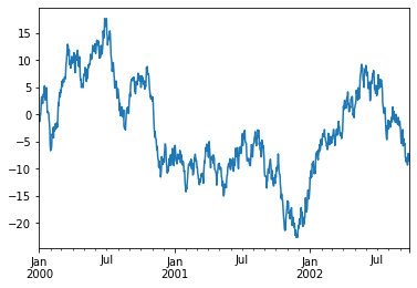
ts = pd.Series(np.random.randn(1000), index=pd.date_range('1/1/2000', periods=1000))
ts = ts.cumsum()
ts.plot()
<AxesSubplot:>
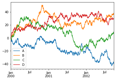
On DataFrame, plot() is a convenience to plot all of the columns with labels:
df = pd.DataFrame(np.random.randn(1000, 4), index=ts.index,
                  columns=['A', 'B', 'C', 'D'])
df = df.cumsum()
plt.figure(); df.plot(); plt.legend(loc='best')
<matplotlib.legend.Legend at 0x7fd7e8a55cd0>


<Figure size 432x288 with 0 Axes>
Getting Data In/Out
CSV
df.to_csv('foo.csv')
pd.read_csv('foo.csv')
| Unnamed: 0 | A | B | C | D | |
|---|---|---|---|---|---|
| 0 | 2000-01-01 | 0.384817 | 0.513609 | -1.705235 | 1.399450 |
| 1 | 2000-01-02 | -1.177765 | -0.886053 | -1.922768 | 1.704903 |
| 2 | 2000-01-03 | -2.197236 | -0.092119 | -1.403218 | 2.196858 |
| 3 | 2000-01-04 | -2.374139 | 0.518876 | -2.551855 | 1.828393 |
| 4 | 2000-01-05 | -3.560139 | 2.067079 | -2.901068 | 2.602319 |
| ... | ... | ... | ... | ... | ... |
| 995 | 2002-09-22 | -37.367730 | 35.506805 | 7.181577 | 29.633260 |
| 996 | 2002-09-23 | -37.688242 | 36.428275 | 7.138265 | 29.185347 |
| 997 | 2002-09-24 | -37.739469 | 37.258316 | 7.570954 | 29.158169 |
| 998 | 2002-09-25 | -38.741428 | 38.066170 | 6.919066 | 30.099116 |
| 999 | 2002-09-26 | -40.062920 | 37.444626 | 7.426596 | 29.419724 |
1000 rows × 5 columns
HDF5
Reading and writing to HDFStores
Writing to a HDF5 Store
df.to_hdf('foo.h5','df')
Reading from a HDF5 Store
pd.read_hdf('foo.h5','df')
| A | B | C | D | |
|---|---|---|---|---|
| 2000-01-01 | 0.384817 | 0.513609 | -1.705235 | 1.399450 |
| 2000-01-02 | -1.177765 | -0.886053 | -1.922768 | 1.704903 |
| 2000-01-03 | -2.197236 | -0.092119 | -1.403218 | 2.196858 |
| 2000-01-04 | -2.374139 | 0.518876 | -2.551855 | 1.828393 |
| 2000-01-05 | -3.560139 | 2.067079 | -2.901068 | 2.602319 |
| ... | ... | ... | ... | ... |
| 2002-09-22 | -37.367730 | 35.506805 | 7.181577 | 29.633260 |
| 2002-09-23 | -37.688242 | 36.428275 | 7.138265 | 29.185347 |
| 2002-09-24 | -37.739469 | 37.258316 | 7.570954 | 29.158169 |
| 2002-09-25 | -38.741428 | 38.066170 | 6.919066 | 30.099116 |
| 2002-09-26 | -40.062920 | 37.444626 | 7.426596 | 29.419724 |
1000 rows × 4 columns
Excel
Reading and writing to MS Excel
Writing to an excel file
df.to_excel('foo.xlsx', sheet_name='Sheet1')
Reading from an excel file
pd.read_excel('foo.xlsx', 'Sheet1', index_col=None, na_values=['NA'])
| Unnamed: 0 | A | B | C | D | |
|---|---|---|---|---|---|
| 0 | 2000-01-01 | 0.384817 | 0.513609 | -1.705235 | 1.399450 |
| 1 | 2000-01-02 | -1.177765 | -0.886053 | -1.922768 | 1.704903 |
| 2 | 2000-01-03 | -2.197236 | -0.092119 | -1.403218 | 2.196858 |
| 3 | 2000-01-04 | -2.374139 | 0.518876 | -2.551855 | 1.828393 |
| 4 | 2000-01-05 | -3.560139 | 2.067079 | -2.901068 | 2.602319 |
| ... | ... | ... | ... | ... | ... |
| 995 | 2002-09-22 | -37.367730 | 35.506805 | 7.181577 | 29.633260 |
| 996 | 2002-09-23 | -37.688242 | 36.428275 | 7.138265 | 29.185347 |
| 997 | 2002-09-24 | -37.739469 | 37.258316 | 7.570954 | 29.158169 |
| 998 | 2002-09-25 | -38.741428 | 38.066170 | 6.919066 | 30.099116 |
| 999 | 2002-09-26 | -40.062920 | 37.444626 | 7.426596 | 29.419724 |
1000 rows × 5 columns
Gotchas
If you are trying an operation and you see an exception like:
if pd.Series([False, True, False]):
    print("I was true")
---------------------------------------------------------------------------

ValueError                                Traceback (most recent call last)

/var/folders/jd/pq0swyt521jb2424d6fvth840000gn/T/ipykernel_71440/2648304181.py in <module>
----> 1 if pd.Series([False, True, False]):
      2     print("I was true")


~/opt/miniconda3/envs/cmu39/lib/python3.9/site-packages/pandas/core/generic.py in __nonzero__(self)
   1535     @final
   1536     def __nonzero__(self):
-> 1537         raise ValueError(
   1538             f"The truth value of a {type(self).__name__} is ambiguous. "
   1539             "Use a.empty, a.bool(), a.item(), a.any() or a.all()."


ValueError: The truth value of a Series is ambiguous. Use a.empty, a.bool(), a.item(), a.any() or a.all().
See Comparisons for an explanation and what to do.
See Gotchas as well.